Added 30/06/2025
Machine Learning / regression
svr_bennett2006
Datasets
Description
Predict car fuel consumption in miles per gallon.Dimension
{
  "x": 19,
  "y": 804,
  "F": 1,
  "G": 11,
  "H": 0,
  "f": 1,
  "g": 2388,
  "h": 0
}
Solution
{
  "optimality": "best_known",
  "F": 2.542799337786741,
  "f": 560.6818881929104,
  "training_r2": 0.8156,
  "training_rmse": 3.3469,
  "validation_r2": 0.8063,
  "validation_rmse": 3.4233
}Dimension
{
  "x": 23,
  "y": 36528,
  "F": 1,
  "G": 13,
  "H": 0,
  "f": 1,
  "g": 109554,
  "h": 0
}
Solution
{
  "optimality": "unknown"
}Description
Predict the median value homes across 507 Boston suburbs and towns.Dimension
{
  "x": 29,
  "y": 1047,
  "F": 1,
  "G": 16,
  "H": 0,
  "f": 1,
  "g": 3102,
  "h": 0
}
Solution
{
  "optimality": "best_known",
  "F": 3.3326596397696857,
  "f": 7476.917189914676,
  "training_r2": 0.7059,
  "training_rmse": 4.9679,
  "validation_r2": 0.6882,
  "validation_rmse": 5.0904
}Description
Predict power plant energy output in MW.Dimension
{
  "x": 13,
  "y": 19149,
  "F": 1,
  "G": 8,
  "H": 0,
  "f": 1,
  "g": 57432,
  "h": 0
}
Solution
{
  "optimality": "best_known",
  "F": 3.6181565191001983,
  "f": 352755.1777047886,
  "training_r2": 0.9282,
  "training_rmse": 4.5724,
  "validation_r2": 0.9281,
  "validation_rmse": 4.5769
}Dimension
{
  "x": 21,
  "y": 2085,
  "F": 1,
  "G": 12,
  "H": 0,
  "f": 1,
  "g": 6228,
  "h": 0
}
Solution
{
  "optimality": "best_known",
  "F": 8.410920349854226,
  "f": 40961.88732629,
  "training_r2": 0.5868,
  "training_rmse": 10.6989,
  "validation_r2": 0.5338,
  "validation_rmse": 11.3674
}Description
Angeliki Xifara, Athanasios TsanasDimension
{
  "x": 21,
  "y": 1563,
  "F": 1,
  "G": 12,
  "H": 0,
  "f": 1,
  "g": 4662,
  "h": 0
}
Solution
{
  "optimality": "unknown"
}Dimension
{
  "x": 21,
  "y": 2703,
  "F": 1,
  "G": 12,
  "H": 0,
  "f": 1,
  "g": 8082,
  "h": 0
}
Solution
{
  "optimality": "best_known",
  "F": 4235.435897403506,
  "f": 654856406585.5027,
  "training_r2": 0.7521,
  "training_rmse": 6025.446,
  "validation_r2": 0.7442,
  "validation_rmse": 6117.632
}Dimension
{
  "x": 17,
  "y": 849,
  "F": 1,
  "G": 10,
  "H": 0,
  "f": 1,
  "g": 2526,
  "h": 0
}
Solution
{
  "optimality": "best_known",
  "F": 6.249691447590366,
  "f": 332723134.5306423,
  "training_r2": 0.5849,
  "training_rmse": 8.7481,
  "validation_r2": 0.5737,
  "validation_rmse": 8.8433
}Description
label = 3.0 * feature_1 - 5.0 * feature_2 + 7.0Dimension
{
  "x": 9,
  "y": 189,
  "F": 1,
  "G": 6,
  "H": 0,
  "f": 1,
  "g": 558,
  "h": 0
}
Solution
{
  "optimality": "global",
  "x": [2.342384984711291,0.00015339162591163628,0,3,-5,7,3,-5,7],
  "F": 0,
  "G": [2.342384984711291,0.00015339162591163628,0,0,0,0],
  "f": 124.5,
  "training_r2": 1,
  "training_rmse": 0,
  "validation_r2": 1,
  "validation_rmse": 0
}Description
label = 1.0 * feature_1 + 2.0 * feature_2 + 3.0 * feature_3 + 4.0 * feature_4 + 6.0 * feature_5 + noiseDimension
{
  "x": 15,
  "y": 1014,
  "F": 1,
  "G": 9,
  "H": 0,
  "f": 1,
  "g": 3024,
  "h": 0
}
Solution
{
  "optimality": "best_known",
  "F": 0.00263100032236596,
  "G": [5.456725485601478,0.005762487216478602,0,0.00008218272962301487,0.000060373800451429815,0.000025519346953828403,0.0005300154736520568,0.000017213393981307945,0.00033956244660801745],
  "f": 82.529647524697,
  "training_r2": 1,
  "training_rmse": 0.0031,
  "validation_r2": 1,
  "validation_rmse": 0.0031
}Dimension
{
  "x": 25,
  "y": 2031,
  "F": 1,
  "G": 14,
  "H": 0,
  "f": 1,
  "g": 6060,
  "h": 0
}
Solution
{
  "optimality": "best_known",
  "F": 0.0025794120164338926,
  "f": 7.109020086333578,
  "training_r2": 1,
  "training_rmse": 0.0029,
  "validation_r2": 1,
  "validation_rmse": 0.003
}\subsection{svr\_bennett2006}
\label{subsec:svr_bennett2006}
% Bold characters for w, w lower bound and w upper bound
\newcommand{\w}{\mathbf{w}}
\newcommand{\wlb}{\mathbf{\bar{w}}}
\newcommand{\wub}{\mathbf{\munderbar{w}}}
% Cite Bennett 2006
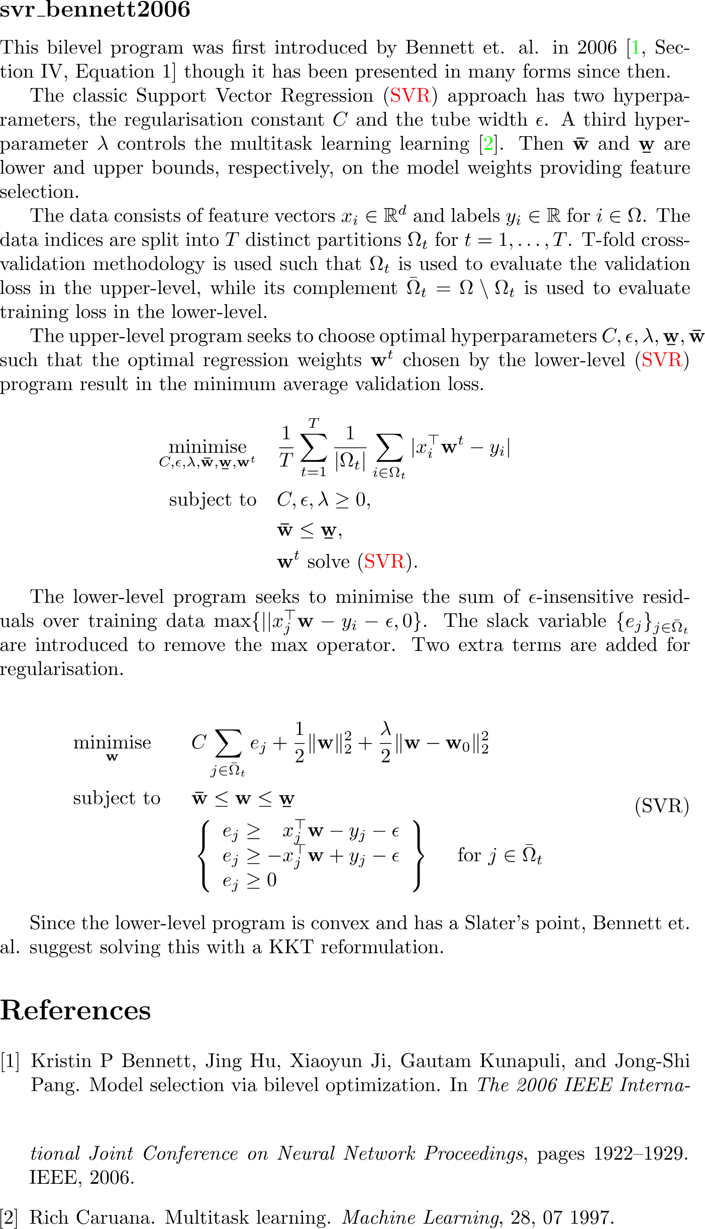
This bilevel program was first introduced by Bennett et. al. in 2006 \cite[Section~IV, Equation~1]{Bennett2006} though it has been presented in many forms since then.
% Introduce the hyperparameters
The classic Support Vector Regression \eqref{eq:svr} approach has two hyperparameters, the regularisation constant $C$ and the tube width $\epsilon$. A third hyperparameter $\lambda$ controls the multitask learning
learning \cite{Caruana1997}. Then $\wlb$ and $\wub$ are lower and upper bounds, respectively, on the model weights providing feature selection.
% T-fold cross-validation split
The data consists of feature vectors $x_i\in\R^d$ and labels $y_i\in\R$ for $i\in\Omega$. The data indices are split into $T$ distinct partitions $\Omega_t$ for $t=1,\dots,T$. T-fold cross-validation methodology is used such that $\Omega_t$ is used to evaluate the validation loss in the upper-level, while its complement $\bar{\Omega}_t=\Omega\setminus\Omega_t$ is used to evaluate training loss in the lower-level.
% Upper-level description
The upper-level program seeks to choose optimal hyperparameters $C,\epsilon,\lambda,\wub,\wlb$ such that the optimal regression weights $\w^t$ chosen by the lower-level \eqref{eq:svr} program result in the minimum average validation loss.
% Upper-level equation
\begin{equation*}
\begin{aligned}
\minimise_{C, \epsilon, \lambda, \wlb, \wub, \w^t} \quad
&\frac{1}{T}\sum_{t=1}^{T} \frac{1}{|\Omega_t|} \sum_{i\in\Omega_t} |x_i^\top\w^t-y_i|&
\\
\subjectto \quad
& C, \epsilon, \lambda \geq 0,& \\
& \wlb \leq \wub,& \\
&\w^t \text{ solve \eqref{eq:svr}}.
\end{aligned}
\end{equation*}
% Lower-level description
The lower-level program seeks to minimise the sum of $\epsilon$-insensitive residuals over training data $\max\{||x_j^\top\w - y_i - \epsilon, 0\}$. The slack variable $\{e_j\}_{j\in\bar{\Omega}_t}$ are introduced to remove the max operator. Two extra terms are added for regularisation.
% Lower-level equation
\begin{align}
\label{eq:svr}
\tag{SVR}
\begin{aligned}
&\minimise_{\w} \quad &
&C\sum_{j\in\bar{\Omega}_t}e_j + \frac{1}{2}\|\w\|_2^2+\frac{\lambda}{2}\|\w-\w_0\|_2^2&
\\
&\subjectto &
& \wlb\leq\w\leq\wub& \\
&&&\left\{
\begin{array}{l}
e_j \geq \phantom{-}x_j^\top\w - y_j - \epsilon\\
e_j \geq -x_j^\top\w + y_j - \epsilon\\
e_j \geq 0
\end{array}
\right\}\quad \text{ for } j\in\bar{\Omega}_t&
\end{aligned}
\end{align}
Since the lower-level program is convex and has a Slater's point, Bennett et. al. suggest solving this with a KKT reformulation.classdef svr_bennett2006
%{
Kristin P Bennett, Jing Hu, Xiaoyun Ji, Gautam Kunapuli, and Jong-Shi Pang.
Model selection via bilevel optimization.
In the 2006 IEEE International Joint Conference on Neural Network Proceedings, pages 1922–1929.
%}
properties(Constant)
name = 'svr_bennett2006';
category = 'machine_learning';
subcategory = 'regression';
T_folds = 3;
datasets = {
'egression_auto_mpg.csv';
'egression_avocado_price.csv';
'egression_boston_house_price.csv';
'egression_combined_cycle_power_plant.csv';
'regression_concrete_compressive_strength.csv';
'regression_energy_efficiency.csv';
'regression_insurance.csv';
'regression_real_estate_valuation.csv';
'regression_toy_2_features.csv';
'regression_toy_5_features.csv';
'regression_toy_10_features.csv';
'regression_toy_20_features.csv';
};
paths = fullfile('bolib3', 'data', 'regression', svr_bennett2006.datasets);
end
methods(Static)
% //==================================================\\
% || F ||
% \\==================================================//
% Upper-level objective function (convex)
% Computes sum over folds of sum_i | Xw - y |
function obj = F(~, y, data)
obj = 0;
d = data.d;
for t = 1:svr_bennett2006.T_folds
w_t = y((t-1)*d + 1 : t*d);
residual = data.val_features{t} * w_t - data.val_labels{t};
obj = obj + (sum(abs(residual))/length(data.val_labels{t}));
end
obj = obj / svr_bennett2006.T_folds;
end
% //==================================================\\
% || G ||
% \\==================================================//
% Upper-level inequality constraints (linear)
% C >= 0
% epsilon >= 0
% lambda >= 0
% w_ub - w_lb >= 0
function val = G(x, ~, data)
d = data.d;
% C, epsilon, lambda >= 0
hp_nonnegativity = x(1:3);
% w_lb <= w_ub => w_ub - w_lb >= 0
w_lb = x(4 : 3 + d);
w_ub = x(4 + d : 3 + 2*d);
w_bounds = w_ub - w_lb;
% Stack them into one vector
val = [hp_nonnegativity; w_bounds];
end
% //==================================================\\
% || H ||
% \\==================================================//
% Upper-level equality constraints (none)
function val = H(~, ~, ~)
val = [];
end
% //==================================================\\
% || f ||
% \\==================================================//
% Lower-level objective function (quadratic)
% obj = sum_t [ C * sum(e_t) + 0.5 * w_t'w_t + lambda * w_t'w_t ]
function obj = f(x, y, data)
% Split variables
[hp_C, ~, hp_lambda, ~, ~, w, e] = svr_bennett2006.variable_split(x, y, data);
obj = 0;
for t = 1:svr_bennett2006.T_folds
obj = obj + hp_C * sum(e{t}) + 0.5 * (w{t}' * w{t}) + hp_lambda * (w{t}' * w{t});
end
end
% //==================================================\\
% || g ||
% \\==================================================//
% Lower-level inequality constraints (linear)
% For each fold t=1,...,T:
% e_j >= + w*x_j - y_j - epsilon
% e_j >= - w*x_j + y_j - epsilon
% e_j >= 0
% w >= w_lb
% w <= w_ub
function constraints = g(x, y, data)
% Split variables
[~, hp_epsilon, ~, w_lb, w_ub, w, e] = svr_bennett2006.variable_split(x, y, data);
% Store all constraints in a cell array
cells = cell(1, 5*svr_bennett2006.T_folds);
for t = 1:svr_bennett2006.T_folds
cells{5*(t-1) + 1} = e{t} + hp_epsilon - (data.train_features{t} * w{t}) + data.train_labels{t};
cells{5*(t-1) + 2} = e{t} + hp_epsilon + (data.train_features{t} * w{t}) - data.train_labels{t};
cells{5*(t-1) + 3} = e{t};
cells{5*(t-1) + 4} = w{t} - w_lb;
cells{5*(t-1) + 5} = w_ub - w{t};
end
% Concatenate all constraints into a single vector
constraints = vertcat(cells{:});
end
% //==================================================\\
% || h ||
% \\==================================================//
% Lower-level equality constraints
function val = h(~, ~, ~)
val = [];
end
% //==================================================\\
% || Variable Split ||
% \\==================================================//
% Upper-level variables:
% x = [C, epsilon, lambda, w_lb, w_ub]
% Lower-level variables:
% y = [w[0], ..., w[T], e[0], ..., e[T]]
%
function [hp_C, hp_epsilon, hp_lambda, w_lb, w_ub, w, e] = variable_split(x, y, data)
% Dimensions
d = data.d;
n_train = data.n_train;
% Upper-level decision variables
hp_C = x(1);
hp_epsilon = x(2);
hp_lambda = x(3);
w_lb = x(4 : 3 + d);
w_ub = x(4 + d : 3 + 2*d);
% Lower-level decision variables
w = cell(1, svr_bennett2006.T_folds);
e = cell(1, svr_bennett2006.T_folds);
for t = 1:svr_bennett2006.T_folds
idx_w_start = (t-1)*d + 1;
idx_w_end = t*d;
w{t} = y(idx_w_start : idx_w_end);
idx_e_start = svr_bennett2006.T_folds*d + (t-1)*n_train + 1;
idx_e_end = svr_bennett2006.T_folds*d + t*n_train;
e{t} = y(idx_e_start : idx_e_end);
end
end
% //==================================================\\
% || Evaluate ||
% \\==================================================//
% Calculates the R2 and RMSE scores of the regression models represented by each fold
function evaluate(~, y, data)
d = data.d;
% Print table headers
fprintf('| %10s | %4s | %10s | %10s | %10s |\n', '', 'fold', 'data', 'R2 score', 'RMSE');
fprintf('| %s | %s | %s | %s | %s |\n', repmat('-',1,10), repmat('-',1,4), repmat('-',1,10), repmat('-',1,10), repmat('-',1,10));
% Evaluate for training and validation folds
tasks = {'Training', 'Validation'};
features_list = {data.train_features, data.val_features};
labels_list = {data.train_labels, data.val_labels};
for idx = 1:2
for t = 1:svr_bennett2006.T_folds
w_t = y((t-1)*d + 1 : t*d);
features = features_list{idx}{t};
labels = labels_list{idx}{t};
predictions = features * w_t;
% RMSE
rmse = sqrt(mean((labels - predictions).^2));
% R2 score
ss_res = sum((labels - predictions).^2);
ss_tot = sum((labels - mean(labels)).^2);
r2 = 1 - ss_res / ss_tot;
% Display
fprintf('| %-10s | %4d | %10s | %10.4f | %10.4f |\n', ...
tasks{idx}, t, sprintf('%dx%d', size(features,1), size(features,2)), r2, rmse);
end
end
end
% //==================================================\\
% || Read Data ||
% \\==================================================//
% The CSV file should have:
% - First row: headers (e.g. 'label', 'feature1', 'feature2', ...)
% - First column: labels (independent variable)
% - Remaining columns: features (dependent variables)
%
% Splits the data into T training and validation folds.
% If len(data) is not divisible by T then the last (len(data)%T) examples are dropped.
% For example consider the dataset [1,...,17] and parameter T is set to 3.
% The procedure can be visualized with the following table:
%
% | | i=1,2,3,4,5 | i=6,7,8,9,10 | i=11,12,13,14,15 |
% |-----|------------------|------------------|------------------|
% | t=1 | validation | train | train |
% | t=2 | train | validation | train |
% | t=3 | train | train | validation |
function data = read_data(filepath)
% Read the csv
options = detectImportOptions(filepath);
data_table = readtable(filepath, options);
% Add a column of ones for the constant term
data_table.constant = ones(height(data_table),1);
% Total number of folds
T = svr_bennett2006.T_folds;
% Extract labels and features
labels = table2array(data_table(:,1));
features = table2array(data_table(:,2:end));
% dimension (total number must be divsible by T)
n_val = floor(length(labels) / T);
n_total = n_val * T;
n_train = n_total - n_val;
% Preallocate cells
val_features = cell(1, T);
val_labels = cell(1, T);
train_features = cell(1, T);
train_labels = cell(1, T);
% Form validation and training sets for each fold t=1,...,T
for t = 1:T
val_indices_t = ((t-1)*n_val + 1):t*n_val;
train_indices_t = setdiff(1:n_total, val_indices_t);
val_features{t} = features(val_indices_t, :);
val_labels{t} = labels(val_indices_t);
train_features{t} = features(train_indices_t, :);
train_labels{t} = labels(train_indices_t);
end
% Form output struct
data = struct();
data.file = filepath;
data.d = size(features, 2);
data.n_val = n_val;
data.val_features = val_features;
data.val_labels = val_labels;
data.n_train = n_train;
data.train_features = train_features;
data.train_labels = train_labels;
end
% Key are the function/variable names
% Values are their dimension
function n = dimension(key, data)
n = dictionary( ...
'x', 3 + 2*data.d, ...
'y', svr_bennett2006.T_folds*(data.d + data.n_train), ...
'F', 1, ...
'G', 3 + data.d, ...
'H', 0, ...
'f', 1, ...
'g', svr_bennett2006.T_folds*(2*data.d + 3*data.n_train), ...
'h', 0 ...
);
if isKey(n,key)
n = n(key);
end
end
end
endimport math
import os
from bolib3 import np
import pandas as pd
"""
Kristin P Bennett, Jing Hu, Xiaoyun Ji, Gautam Kunapuli, and Jong-Shi Pang.
Model selection via bilevel optimization.
In the 2006 IEEE International Joint Conference on Neural Network Proceedings, pages 1922–1929.
"""
# Properties
name: str = "svr_bennett2006"
category: str = "machine_learning"
subcategory: str = "regression"
T_folds: int = 3
datasets: list = [
"regression_auto_mpg.csv",
"regression_avocado_price.csv",
"regression_boston_house_price.csv",
"regression_combined_cycle_power_plant.csv",
'regression_concrete_compressive_strength.csv',
"regression_energy_efficiency.csv",
"regression_insurance.csv",
"regression_real_estate_valuation.csv",
"regression_toy_2_features.csv",
"regression_toy_5_features.csv",
"regression_toy_10_features.csv",
"regression_toy_20_features.csv",
]
paths: list = [
os.path.join("bolib3", "data", "regression", dataset) for dataset in datasets
]
# //==================================================\\
# || F ||
# \\==================================================//
def F(x, y, data):
"""
Upper-level objective function (convex)
sum_{t} sum_{i} | (val_features_{ti} * w_{t} - val_labels_{ti}) |
"""
obj = 0
for t in range(T_folds):
w_t = y[t*data['d']: (t + 1)*data['d']]
residuals = np.abs(np.dot(data['val_features'][t], w_t) - data['val_labels'][t])
obj += np.sum(residuals)/len(data['val_labels'][t])
return obj / T_folds
# //==================================================\\
# || G ||
# \\==================================================//
def G(x, y, data=None):
"""
Upper-level inequality constraints (linear)
C >= 0
epsilon >= 0
lambda >=0
w_lb <= w_ub
"""
d = data['d']
return np.concatenate([
x[0:3],
x[3 + d:3 + 2*d] - x[3:3 + d]
])
# //==================================================\\
# || H ||
# \\==================================================//
def H(x, y, data=None):
"""
Upper-level equality constraints (none)
"""
return np.empty(0)
# //==================================================\\
# || f ||
# \\==================================================//
def f(x, y, data=None):
"""
Lower-level objective function (quadratic)
"""
hp_C, hp_epsilon, hp_lambda, w_lb, w_ub, w, e = variable_split(x, y, data)
obj = 0
for t in range(T_folds):
obj += hp_C*np.sum(e[t]) + 0.5*np.dot(w[t], w[t]) + hp_lambda*np.dot(w[t], w[t])
return obj
# //==================================================\\
# || g ||
# \\==================================================//
def g(x, y, data=None):
"""
Lower-level inequality constraints (linear)
e_j >= + w * x_j - y_j - epsilon
e_j >= - w * x_j + y_j - epsilon
e_j >= 0
"""
hp_C, hp_epsilon, hp_lambda, w_lb, w_ub, w, e = variable_split(x, y, data)
constraints = []
for t in range(T_folds):
constraints.append(e[t] + hp_epsilon - np.dot(data['train_features'][t], w[t]) + data['train_labels'][t])
constraints.append(e[t] + hp_epsilon + np.dot(data['train_features'][t], w[t]) - data['train_labels'][t])
constraints.append(e[t])
constraints.append(w[t] - w_lb)
constraints.append(w_ub - w[t])
return np.concatenate(constraints)
# //==================================================\\
# || h ||
# \\==================================================//
def h(x, y, data=None):
"""
Lower-level equality constraints (none)
"""
return np.empty(0)
# //==================================================\\
# || Variable Split ||
# \\==================================================//
def variable_split(x, y, data):
"""
Splits the vectors x, y into their more meaningful components.
Upper-level variables: x = (C, epsilon, lambda, w_lb, w_ub).
Lower-level variables: y = (w[0], ..., w[T], e[0], ..., e[T]).
"""
# Dimensions of the data
d = data['d']
n_train = data['n_train']
# Upper-level decision variables
hp_C = x[0] # C regularisation hyperparameter
hp_epsilon = x[1] # epsilon tube width hyperparameter
hp_lambda = x[2] # lambda multi task learning hyperparameter
w_lb = x[3:3 + d] # w lower bound
w_ub = x[3 + d:3 + 2*d] # w upper bound
# Lower-level decision variables
w = [None]*T_folds
e = [None]*T_folds
for t in range(0, T_folds):
w[t] = y[t*d: (t + 1)*d]
e[t] = y[T_folds*d + t*n_train: T_folds*d + (t + 1)*n_train]
return hp_C, hp_epsilon, hp_lambda, w_lb, w_ub, w, e
# //==================================================\\
# || Variable Join ||
# \\==================================================//
def variable_join(hp_C, hp_epsilon, hp_lambda, w, data):
"""
Joins the variables into
Upper-level variables: x = (C, epsilon, lambda, w_lb, w_ub).
Lower-level variables: y = (w[0], ..., w[T], e[0], ..., e[T]).
"""
w_lb = np.min(w, axis=0)
w_ub = np.max(w, axis=0)
e = []
for t in range(T_folds):
e.append(
np.max(
[
np.dot(data['train_features'][t], w[t]) - data['train_labels'][t] - hp_epsilon,
- np.dot(data['train_features'][t], w[t]) + data['train_labels'][t] - hp_epsilon,
np.zeros(data['n_train'])
],
axis=0
)
)
x = np.concatenate([[hp_C, hp_epsilon, hp_lambda], w_lb, w_ub])
y = np.concatenate(w + e)
return x, y
# //==================================================\\
# || Evaluate ||
# \\==================================================//
def evaluate(x, y, data):
"""
Calculates the R2 and RMSE scores of the regression models represented by each fold
"""
# Print table headers
print(f"| {'':^10} | {'fold':^4} | {'data':^10} | {'R2 score':^10} | {'RMSE':^10} |")
print(f"| {'':-^10} | {'':-^4} | {'':-^10} | {'':-^10} | {'':-^10} |")
# Iterate over first training and then validation T-folds
for task, features, observations in (
('Training', data['train_features'], data['train_labels']),
('Validation', data['val_features'], data['val_labels'])
):
rmse_sum = 0
r2_sum = 0
for t in range(T_folds):
# Make predictions on the data
w_t = y[t*data['d']: (t + 1)*data['d']]
predictions_t = np.dot(features[t], w_t)
# Score RMSE and R2
rmse = np.sqrt(np.mean((observations[t] - predictions_t)**2))
r2 = 1 - (
np.sum((observations[t] - predictions_t)**2)/
np.sum((observations[t] - np.mean(observations[t]))**2)
)
# Output results for fold t
print(f"| {task:<10} | {t:^4} | {str(features[t].shape):^10} | {r2:^10.4f} | {rmse:^10.4f} |")
# Add them to the sum
rmse_sum += rmse
r2_sum += r2
# Output mean results
print(f"| {task:<10} | {'mean':^4} | {'':^10} | {r2_sum/T_folds:^10.4f} | {rmse_sum/T_folds:^10.4f} |")
# //==================================================\\
# || Read Data ||
# \\==================================================//
def read_data(filepath=datasets[0]):
"""
The CSV file should have:
- First row: headers (e.g. 'label', 'feature1', 'feature2', ...)
- First column: labels (independent variable)
- Remaining columns: features (dependent variables)
Splits the data into T training and validation folds.
If len(data) is not divisible by T then the last (len(data)%T) examples are dropped.
For example consider the dataset X=[1,...,17] and parameter T is set to 3.
The procedure can be visualized with the following table:
| | j=1,2,3,4,5 | j=6,7,8,9,10 | j=11,12,13,14,15 |
|-----|------------------|------------------|------------------|
| t=1 | validation | train | train |
| t=2 | train | validation | train |
| t=3 | train | train | validation |
"""
# Read the csv
df = pd.read_csv(filepath)
# Add a column of ones
df['constant'] = 1.0
# Don't Shuffle as this breaks the deterministic setup!!
# df = df.sample(frac=1, random_state=0).reset_index(drop=True)
# Total number of folds is
T = T_folds
# Extract features and label
labels = np.array(df.iloc[:, 0].values)
features = np.array(df.iloc[:, 1:].values)
# Validation Data
n_val = math.floor(len(labels)/T)
val_features = [features[t*n_val:(t + 1)*n_val] for t in range(T)]
val_labels = [labels[t*n_val:(t + 1)*n_val] for t in range(T)]
# Training data
n_train = n_val*(T - 1)
train_features = [np.concatenate(
[features[t_*n_val:(t_ + 1)*n_val] for t_ in range(T) if t_ != t]
) for t in range(T)]
train_labels = [np.concatenate(
[labels[t_*n_val:(t_ + 1)*n_val] for t_ in range(T) if t_ != t]
) for t in range(T)]
# Form into a dictionary
data = {
"path": filepath,
'd': features.shape[1],
"n_val": n_val,
"val_features": val_features,
"val_labels": val_labels,
"n_train": n_train,
"train_features": train_features,
"train_labels": train_labels,
}
return data
# //==================================================\\
# || Dimension ||
# \\==================================================//
def dimension(key='', data=None):
"""
If the argument 'key' is not specified, then:
- a dictionary mapping variable/function names (str) to the corresponding dimension (int) is returned.
If the first argument 'key' is specified, then:
- a single integer representing the dimension of the variable/function with the name {key} is returned.
"""
d = data['d']
n_train = data['n_train']
n = {
"x": 3 + 2*d,
"y": T_folds*(d + n_train),
"F": 1,
"G": 3 + d,
"H": 0,
"f": 1,
"g": T_folds*(3*n_train + 2*d),
"h": 0,
}
if key in n:
return n[key]
return n
# Feasible point
x0 = np.array([
942.69, # C
1.10, # Epsilon
394.61, # Lambda
0.00, -0.81, -0.04, -0.01, -0.38, 0.57, 1.29, -3.18, # w lower bound
0.02, -0.33, -0.01, -0.00, 0.09, 0.64, 1.37, -3.18 # w upper bound
])
x0 = np.array([
1.0, # C
1.0, # Epsilon
1.0, # Lambda
0.00615244, -0.8459975, -0.08478079, -0.00612273, -0.2105129, 0.50659832, 0.85530825, -0.49095779, # w lower bound
0.01608997, -0.08182366, -0.00441689, -0.00474096, -0.09918633, 0.65285064, 1.50846709, 0.15002266, # w upper bound
])
x0 = np.array([
1.0, # C
1.0, # Epsilon
1.0, # Lambda
999, 999, 999, 999, 999, 999, 999, 999, 999, 999, 999, 999, 999, # w lower bound
-999, -999, -999, -999, -999, -999, -999, -999, -999, -999, -999, -999, -999 # w upper bound
])