Added 30/06/2025
Machine Learning / classification
svm_ward2025
Datasets
Description
Coordinates of a positive class encircled by a negative class.Dimension
{
  "x": 92,
  "y": 180,
  "F": 1,
  "G": 182,
  "H": 0,
  "f": 1,
  "g": 360,
  "h": 3
}
Solution
{
  "optimality": "best_known",
  "F": 0.13757920381634928,
  "f": -229817.18253128804,
  "training_accuracy": 1,
  "validation_accuracy": 1
}Description
The elements of statistical learning: data mining, inference, and prediction https://doi.org/10.1007/978-0-387-84858-7Dimension
{
  "x": 92,
  "y": 180,
  "F": 1,
  "G": 182,
  "H": 0,
  "f": 1,
  "g": 360,
  "h": 3
}
Solution
{
  "optimality": "best_known",
  "F": 0.39193660651449896,
  "f": -528677.0555188758,
  "training_accuracy": 1,
  "validation_accuracy": 0.8667
}Description
Antennas radar signals used to classify structure in the ionosphere.Dimension
{
  "x": 122,
  "y": 240,
  "F": 1,
  "G": 242,
  "H": 0,
  "f": 1,
  "g": 480,
  "h": 3
}
Solution
{
  "optimality": "best_known",
  "F": 0.3319446333333333,
  "f": -369.06116861352183,
  "training_accuracy": 0.975,
  "validation_accuracy": 0.8917
}Description
Length and width of sepals and petals labelled by species.Dimension
{
  "x": 101,
  "y": 198,
  "F": 1,
  "G": 200,
  "H": 0,
  "f": 1,
  "g": 396,
  "h": 3
}
Solution
{
  "optimality": "stationary",
  "F": 0.018722626262626264,
  "f": -5.9342439,
  "training_accuracy": 1,
  "validation_accuracy": 1
}Description
Linearly Separable 2d dataset.Dimension
{
  "x": 32,
  "y": 60,
  "F": 1,
  "G": 62,
  "H": 0,
  "f": 1,
  "g": 120,
  "h": 3
}
Solution
{
  "optimality": "best_known",
  "F": 0.012538136666666666,
  "f": -14.804825791886108,
  "training_accuracy": 0,
  "validation_accuracy": 0
}Description
Coordinates sampled from two interweaving crescent moons.Dimension
{
  "x": 56,
  "y": 108,
  "F": 1,
  "G": 110,
  "H": 0,
  "f": 1,
  "g": 216,
  "h": 3
}
Solution
{
  "optimality": "stationary",
  "F": 0,
  "f": -129.60947,
  "training_accuracy": 1,
  "validation_accuracy": 1
}Description
Observations of penguins used to classify their species.Dimension
{
  "x": 266,
  "y": 528,
  "F": 1,
  "G": 530,
  "H": 0,
  "f": 1,
  "g": 1056,
  "h": 3
}
Solution
{
  "optimality": "best_known",
  "F": 0.06366770811027671,
  "f": -1199.3501212164178,
  "training_accuracy": 1,
  "validation_accuracy": 0.9848
}\subsection{svm\_ward2025}
\label{subsec:svm_ward2025}
% Notation.
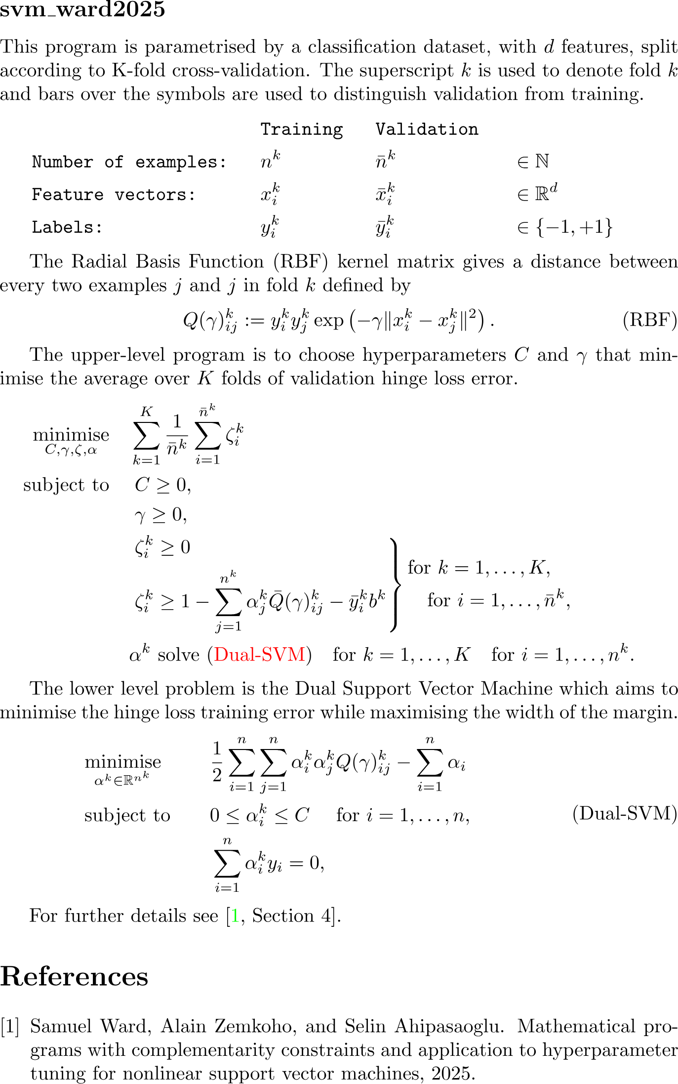
This program is parametrised by a classification dataset, with $d$ features, split according to K-fold cross-validation.
The superscript $k$ is used to denote fold $k$ and bars over the symbols are used to distinguish validation from training.
\begin{subequations}
\begin{align*}
% Titles
&&
&\texttt{Training}&
&\texttt{Validation}&\notag\\
% n
&\texttt{Number of examples:}&
&n^{k}&
&\bar{n}^{k}&
&\in\N&\\
% Feature vector
&\texttt{Feature vectors:}&
&x_i^{k}&
&\bar{x}_i^{k}&
&\in\R^d&\\
% Label
&\texttt{Labels:}&
&y_i^{k}&
&\bar{y}_i^{k}&
&\in\{-1,+1\}&
\end{align*}
\end{subequations}
% RBF
The Radial Basis Function (RBF) kernel matrix gives a distance between every two examples $j$ and $j$ in fold $k$ defined by
\begin{equation*}
\tag{RBF}
\label{eq:rbf}
{Q}(\gamma)^k_{ij}:={y}_i^k y_j^k \exp\left(-\gamma\|{x}^k_i-x^k_j\|^2\right).
\end{equation*}
% Upper-level program
The upper-level program is to choose hyperparameters $C$ and $\gamma$ that minimise the average over $K$ folds of validation hinge loss error.
\begin{equation*}
\begin{aligned}
\minimise_{C, \gamma, \zeta, \alpha} \quad
&\sum_{k=1}^{K} \frac{1}{\bar{n}^k} \sum_{i=1}^{\bar{n}^k} \zeta_i^k&
\\
\subjectto \quad
&\left. C \geq 0, \right.& \\
&\left. \gamma \geq 0, \right.& \\
% Validation
&\left.
\begin{aligned}
&\zeta_i^k \geq 0 \quad \quad \quad \\
&\zeta_i^k \geq 1-\sum_{j=1}^{n^k} \alpha{_j^k} \bar{Q}(\gamma)^k_{ij} - \bar{y}_i^k b^k\\
\end{aligned}
\right\}
\begin{aligned}
&\text{for }k=1,\hdots,K,\\
&\quad\text{for }{i=1,\hdots,\bar{n}^k},
\end{aligned}
\\
% Training
&\alpha^k \text{ solve \eqref{eq:dual_svm}}
\quad \text{for }k=1,\hdots,K\quad\text{for } {i=1,\hdots,n^k}.
\end{aligned}
\end{equation*}
% Lower-level program
The lower level problem is the Dual Support Vector Machine which aims to minimise the hinge loss training error while maximising the width of the margin.
\begin{align}
\label{eq:dual_svm}
\tag{Dual-SVM}
\begin{aligned}
&\minimise_{\alpha{^k} \in \R^{n^k}} \quad &
&\frac{1}{2} \sum_{i=1}^{n} \sum_{j=1}^{n} \alpha{^k_i} \alpha{^k_j} Q(\gamma)^k_{ij} - \sum_{i=1}^{n} \alpha{_i}&
\\
&\subjectto \quad &
&0 \leq \alpha{^k_i} \leq C \quad \text{ for } i=1,\dots,n,&
\\
&&
& \sum_{i=1}^n \alpha{^k_i} y_i =0,&
\end{aligned}
\end{align}
% Citation
For further details see~\cite[Section 4]{Ward2025}.classdef svm_ward2025
%{
Samuel Ward, Alain Zemkoho, and Selin Ahipasaoglu.
Mathematical programs with complementarity constraints and application
to hyperparameter tuning for nonlinear support vector machines. 2025.
%}
properties(Constant)
name = 'svm_ward2025';
category = 'machine_learning';
subcategory = 'classification';
K_folds = 3;
datasets = {
'classification_ionosphere.csv';
'classification_circles90.csv';
'classification_hastie2009.csv';
'classification_iris.csv';
'classification_linearly_separable30.csv';
'classification_moons54.csv';
'classification_palmer.csv'
};
paths = fullfile('bolib3', 'data', 'classification', svm_ward2025.datasets);
end
methods(Static)
% //==================================================\\
% || F ||
% \\==================================================//
% Upper-level objective function (linear)
% Sum of the upper-level varaibles from index 3 to end
function val = F(x, ~, ~)
val = sum(x(3:end)) / (length(x) - 2);
end
% //==================================================\\
% || G ||
% \\==================================================//
% Upper-level inequality constraints (nonconvex)
% - C >= 0
% - gamma >= 0
% - zeta >= 0 for all k,i
% - zeta^k_i - 1 + sum_j (alpha^k_j * Q^k_ij) + y^k_i * b >= 0 for each k,i
function ineq = G(x, y, data)
% Number of validation/training examples
n_val = data.n_val;
n_train = data.n_train;
% Upper-level hyperparameters
C = x(1);
gamma = x(2);
% Start with non-negativity of x
ineq = x;
% Loop over folds
for k = 1:svm_ward2025.K_folds
% Index the subvectors for zeta and alpha relating to the k-th fold
idx_zeta = 2 + ((k-1)*n_val) + (1:n_val);
idx_alpha = ((k-1)*n_train) + (1:n_train);
zeta_k = x(idx_zeta);
alpha_k = y(idx_alpha);
% Extract data relating to the k-th fold
train_labels_k = data.train_labels{k};
train_features_k = data.train_features{k};
val_labels_k = data.val_labels{k};
val_features_k = data.val_features{k};
% Calculate the kernel and the bias (depend on the hyperparameters C and gamma)
Q_k = exp(-gamma * svm_ward2025.pairwise_squared_distance_matrix(val_features_k, train_features_k));
bias_k = svm_ward2025.reconstruct_bias(alpha_k, C, gamma, train_features_k, train_labels_k);
% Add the constraint Z
constraint_Z = zeta_k - 1 + (Q_k * (alpha_k .* train_labels_k)) - (val_labels_k * bias_k);
ineq = [ineq; constraint_Z];
end
end
% //==================================================\\
% || H ||
% \\==================================================//
% Upper-level equality constraints (none)
function val = H(~, ~, ~)
val = [];
end
% //==================================================\\
% || f ||
% \\==================================================//
% Lower-level objective function
function obj = f(x, y, data)
gamma = x(2);
obj = 0;
for k = 1:svm_ward2025.K_folds
idx_alpha = ((k-1)*data.n_train) + (1:data.n_train);
alpha_k = y(idx_alpha);
a_times_y = alpha_k .* data.train_labels{k};
Q = exp(-gamma * svm_ward2025.pairwise_squared_distance_matrix(data.train_features{k}, data.train_features{k}));
obj = obj + 0.5 * (a_times_y' * Q * a_times_y) - sum(alpha_k);
end
end
% //==================================================\\
% || g ||
% \\==================================================//
% Lower-level inequality constraints
% 0 <= alpha <= C
function val = g(x, y, ~)
val = [
y(:);
y(:) - x(1)
];
end
% //==================================================\\
% || h ||
% \\==================================================//
% Lower-level equality constraints
% For each fold k=1,...,K:
% sum_{i=1} (aplha(k,i)) * (train_labels(k,i)) == 0
function val = h(~, y, data)
val = zeros(svm_ward2025.K_folds, 1);
% Iterate over the K folds
for k = 1:(svm_ward2025.K_folds)
idx_alpha_k = ((k-1)*data.n_train) + (1:data.n_train);
alpha_k = y(idx_alpha_k);
val(k) = sum(alpha_k .* data.train_labels{k});
end
end
% //==================================================\\
% || Pairwise Squared Distance Matrix ||
% \\==================================================//
% a: [n_a x d]
% b: [n_b x d]
% D: [n_a x n_b] where D(i,j) = ||a_i - b_j||^2
function D = pairwise_squared_distance_matrix(a, b)
% Compute squared norms
a_norm_sq = sum(a.^2, 2);
b_norm_sq = sum(b.^2, 2);
% Pairwise squared distances
D = bsxfun(@plus, a_norm_sq, b_norm_sq') - 2 * (a * b');
end
% //==================================================\\
% || Reconstruct Bias ||
% \\==================================================//
% Compute the SVM bias term from dual variables.
% See Appendix B of Ward 2025.
function b = reconstruct_bias(alpha_k, C, gamma, train_features_k, train_labels_k)
rbf_kernel = exp(-gamma * svm_ward2025.pairwise_squared_distance_matrix(train_features_k, train_features_k));
omega_of_alpha_k = 1 - ((2 * alpha_k / C) - 1).^4 + 1e-5;
sum_term = train_labels_k - (rbf_kernel * (alpha_k .* train_labels_k));
b = dot(omega_of_alpha_k' , sum_term) / sum(omega_of_alpha_k);
end
% //==================================================\\
% || Evaluate ||
% \\==================================================//
% Calculate mean training and validation accuracies for the SVM.
function [mean_train_accuracy, mean_val_accuracy] = evaluate(x, y, data)
train_accuracies = zeros(svm_ward2025.K_folds, 1);
val_accuracies = zeros(svm_ward2025.K_folds, 1);
% Iterate over K folds
for k = 1:svm_ward2025.K_folds
% Make predictions
training_predict = svm_ward2025.predict(x, y, data, k, data.train_features{k});
validation_predict = svm_ward2025.predict(x, y, data, k, data.val_features{k});
% Callcuate accuracy
train_accuracies(k) = sum(training_predict == data.train_labels{k}) / data.n_train;
val_accuracies(k) = sum(validation_predict == data.val_labels{k}) / data.n_val;
end
% Mean accuracies
mean_train_accuracy = mean(train_accuracies);
mean_val_accuracy = mean(val_accuracies);
% Output
fprintf('C: %.2e\n', x(1));
fprintf('gamma: %.2e\n', x(2));
fprintf('Mean training accuracy: %.2f%%\n', mean_train_accuracy * 100);
fprintf('Mean validation accuracy: %.2f%%\n', mean_val_accuracy * 100);
end
% //==================================================\\
% || Predict ||
% \\==================================================//
% Takes the k-th lower-level SVM represented by decision variables (x, y, data)
% Makes classification predictions for unseen_examples
function predictions = predict(x, y, data, k, unseen_examples)
% Hyperparameters C and gamma
C = x(1);
gamma = x(2);
% SVM dual variables for fold k
idx_alpha = ((k-1)*data.n_train) + (1:data.n_train);
alpha_k = y(idx_alpha);
bias_k = svm_ward2025.reconstruct_bias(alpha_k, C, gamma, data.train_features{k}, data.train_labels{k});
% Make predictions
kernel = exp(-gamma * svm_ward2025.pairwise_squared_distance_matrix(unseen_examples, data.train_features{k}));
decision = kernel * (alpha_k .* data.train_labels{k}) + bias_k;
predictions = sign(decision);
end
% //==================================================\\
% || Read Data ||
% \\==================================================//
% Reads a classification dataset from a csv file.
% - First row should contain header names (e.g. 'label', 'feature1', 'feature2', ...)
% - First column should contain +1/-1 labels (e.g. [+1, -1, -1, +1, ...])
%
% Splits the data into K training and validation folds.
% If len(data) is not divisible by K then the last (len(data)%K) examples are dropped.
% For example consider the dataset X=[1,...,17] and parameter K is set to 3.
% The procedure can be visualized with the following table:
%
% | | i=1,2,3,4,5 | i=6,7,8,9,10 | i=11,12,13,14,15 |
% |-----|------------------|------------------|------------------|
% | k=1 | validation | train | train |
% | k=2 | train | validation | train |
% | k=3 | train | train | validation |
function data = read_data(filepath)
% Read CSV as table
data_table = readtable(filepath);
K = svm_ward2025.K_folds;
% Extract labels (first column) and features (remaining columns)
labels = table2array(data_table(:, 1));
features = table2array(data_table(:, 2:end));
% Assertions
if ~all(ismember(labels, [-1, 1]))
error('Data contains labels other than -1 and +1');
end
if size(labels, 1) ~= size(features, 1)
error('Labels and features must have the same number of rows');
end
% Number of examples per fold
n_val = floor(length(labels) / K);
n_train = n_val * (K - 1);
% Preallocate cells
val_features = cell(K, 1);
val_labels = cell(K, 1);
train_features = cell(K, 1);
train_labels = cell(K, 1);
% Split data into folds
for k = 1:K
idx_val = ( (k-1)*n_val + 1 ) : (k*n_val);
val_features{k} = features(idx_val, :);
val_labels{k} = labels(idx_val, :);
idx_train = setdiff(1:(n_val*K), idx_val);
train_features{k} = features(idx_train, :);
train_labels{k} = labels(idx_train, :);
end
% Form struct
data = struct();
data.file = filepath;
data.n_val = n_val;
data.val_features = val_features;
data.val_labels = val_labels;
data.n_train = n_train;
data.train_features = train_features;
data.train_labels = train_labels;
end
% //==================================================\\
% || Dimensions ||
% \\==================================================//
% Key are the function/variable names
% Values are their dimension
function n = dimension(key, data)
n = dictionary( ...
'x', 2 + svm_ward2025.K_folds*data.n_val, ...
'y', svm_ward2025.K_folds*data.n_train, ...
'F', 1, ...
'G', 2 + 2*svm_ward2025.K_folds*data.n_val, ...
'H', 0, ...
'f', 1, ...
'g', 2*svm_ward2025.K_folds*data.n_train, ...
'h', svm_ward2025.K_folds ...
);
if isKey(n,key)
n = n(key);
end
end
end
endimport os.path
from bolib3 import np
import pandas as pd
import math
"""
Samuel Ward, Alain Zemkoho, and Selin Ahipasaoglu.
Mathematical programs with complementarity constraints and application
to hyperparameter tuning for nonlinear support vector machines. 2025.
"""
# Properties
name: str = "svm_ward2025"
category: str = "machine_learning"
subcategory: str = "classification"
K_folds: int = 3
datasets: list = [
'classification_circles90.csv',
'classification_hastie2009.csv',
'classification_ionosphere.csv',
'classification_iris.csv',
'classification_linearly_separable30.csv',
'classification_moons54.csv',
'classification_palmer.csv'
]
paths = [
os.path.join("bolib3", "data", "classification", d) for d in datasets
]
# //==================================================\\
# || F ||
# \\==================================================//
def F(x, y, data):
"""
Upper-level objective function
(linear)
minimise Σ ζ^k_i
"""
return np.sum(x[2:])/(len(x) - 2)
# //==================================================\\
# || G ||
# \\==================================================//
def G(x, y, data=None):
"""
Upper-level inequality constraints
(nonconvex)
C ≥ 0
γ ≥ 0
ζ^k_i ≥ 0 for each k,i
ζ^k_i - 1 + Σ_j ( α^k_j Q^k_ij ) + y^k_i * b ≥ 0 for each k,i
"""
# Hyperparameters C and gamma are the first and second upper-level variables respectively
C = x[0]
gamma = x[1]
# Number of validation and training examples
n_val = data['n_val']
n_train = data['n_train']
# Index zeta and alpha
zeta = [x[2 + k*n_val:2 + (k + 1)*n_val] for k in range(K_folds)]
alpha = [y[k*n_train:(k + 1)*n_train] for k in range(K_folds)]
violation = margin_violation(C, gamma, alpha, data)
# Concatenate the list of inequality constraints and return them as a 1d array
return np.concatenate(
[x] +
[zeta[k] - violation[k] for k in range(K_folds)],
)
# //==================================================\\
# || H ||
# \\==================================================//
def H(x, y, data=None):
"""
Upper-level equality constraints
(none)
"""
return np.empty(0)
# //==================================================\\
# || f ||
# \\==================================================//
def f(x, y, data=None):
"""
Lower-level objective function
(non-linear)
"""
n_train = data['n_train']
gamma = x[1]
# Iterate over the K folds of training data and cumulatively sum the objective
obj = 0
for k in range(K_folds):
# Extract the lower-level decision variables alpha
alpha = y[k*n_train:(k + 1)*n_train]
# Extract the training data for fold k
train_features_k, train_labels_k = data['train_features'][k], data['train_labels'][k]
# Evaluate the training loss
a_times_y = np.multiply(alpha, train_labels_k)
Q = np.exp(-gamma*pairwise_squared_distance_matrix(train_features_k, train_features_k))
obj += 0.5*np.dot(a_times_y, np.dot(Q, a_times_y)) - np.sum(alpha)
# Return the lower-level objective
return obj
# //==================================================\\
# || g ||
# \\==================================================//
def g(x, y, data=None):
"""
Lower-level inequality constraints
0 ≤ α ≤ C
"""
return np.concatenate([y, -y + x[0]])
# //==================================================\\
# || h ||
# \\==================================================//
def h(x, y, data=None):
"""
Lower-level equality constraints
Σ α_i y_i = 0 for each fold
"""
train_labels = data['train_labels']
n_train = data['n_train']
alpha = [y[k*n_train:(k + 1)*n_train] for k in range(K_folds)]
return np.array([
np.dot(alpha[k], train_labels[k]) for k in range(K_folds)
])
# //==================================================\\
# || Margin Violation ||
# \\==================================================//
def margin_violation(C, gamma, alpha, data):
"""
Returns a list index by the folds k=1,...,K.
Each element is a numpy array indexed by i=1,...,n_val.
Such that the element violation[k][i] is given by:
1 - SUM_[j=1,...,n_k] (( α_[k,j] * Q_[k,i,j] )) - y_[k,i] * b
See Ward et al. 2025.
"""
violation = []
for k in range(K_folds):
# Extract the data corresponding to fold k
train_labels_k = data['train_labels'][k]
train_features_k = data['train_features'][k]
val_labels_k = data['val_labels'][k]
val_features_k = data['val_features'][k]
# Calculate the kernel and the bias (depend on the hyperparameters C and gamma)
rbf_kernel_train_val = np.exp(-gamma*pairwise_squared_distance_matrix(train_features_k, val_features_k))
bias = reconstruct_bias(alpha[k], C, gamma, train_features_k, train_labels_k)
# The violation is calculated by 1 - Σ( αj Qij ) - yi b
violation.append(
1 - np.dot(
np.multiply(alpha[k], train_labels_k),
np.multiply(val_labels_k, rbf_kernel_train_val)
) - bias*val_labels_k
)
return violation
# //==================================================\\
# || Split Variables ||
# \\==================================================//
def split_variables(x, y, data):
"""
Split variables into their interpretable components
x = [C, gamma, zeta_(1,1), zeta_(1,2), ..., zeta_(K, n_val)]
y = [alpha_(1,1), alpha_(1,2), ..., alpha_(K, n_train)]
"""
n_val = data['n_val']
n_train = data['n_train']
C = x[0]
gamma = x[1]
zeta = [x[2 + k*n_val:2 + (k + 1)*n_val] for k in range(K_folds)]
alpha = [y[k*n_train:(k + 1)*n_train] for k in range(K_folds)]
return C, gamma, zeta, alpha
# //==================================================\\
# || join variables ||
# \\==================================================//
def join_variables(C, gamma, alpha, data):
"""
Given C, gamma and alpha will construct
(1) Upper-level variable x = [C, gamma, zeta_(1,1), zeta_(1,2), ..., zeta_(K, n_val)]
(2) Lower-level variable y = [alpha_(1,1), alpha_(1,2), ..., alpha_(K, n_train)]
"""
violation = margin_violation(C, gamma, alpha, data)
zeta = [np.fmax(violation[k], 0) for k in range(K_folds)]
x = np.hstack([C] + [gamma] + zeta)
y = np.hstack(alpha)
assert len(x) == dimension('x', data), 'Dimension error'
assert len(y) == dimension('y', data), 'Dimension error'
return x, y
# //==================================================\\
# || Read Data ||
# \\==================================================//
def read_data(filepath=paths[0], verbose=False):
"""
Reads a classification dataset from a csv file.
- First row should contain header names (e.g. 'label', 'feature1', 'feature2', ...)
- First column should contain +1/-1 labels (e.g. [+1, -1, -1, +1, ...])
Splits the data into K training and validation folds.
If len(X) is not divisible by K then the last (len(X)%K) examples are dropped.
For example consider the dataset X=[1,...,17] and parameter K is set to 3.
The procedure can be visualized with the following table:
| | i=1,2,3,4,5 | i=6,7,8,9,10 | i=11,12,13,14,15 |
|-----|------------------|------------------|------------------|
| k=1 | validation | train | train |
| k=2 | train | validation | train |
| k=3 | train | train | validation |
"""
# Read the csv
df = pd.read_csv(filepath)
# Total number of folds is
K = K_folds
# Extract features and label
labels = np.array(df.iloc[:, 0].values)
features = np.array(df.iloc[:, 1:].values)
# Assertions
assert np.all(np.isin(labels, [-1, 1])), "Data contains labels other than -1 and +1"
assert labels.shape[0] == features.shape[0], "Labels and features must have same number of rows"
# Validation Data
n_val = math.floor(len(labels)/K)
val_features = [features[k*n_val:(k + 1)*n_val] for k in range(K)]
val_labels = [labels[k*n_val:(k + 1)*n_val] for k in range(K)]
# Training data
n_train = n_val*(K - 1)
train_features = [np.concatenate(
[features[k_*n_val:(k_ + 1)*n_val] for k_ in range(K) if k_ != k]
) for k in range(K)]
train_labels = [np.concatenate(
[labels[k_*n_val:(k_ + 1)*n_val] for k_ in range(K) if k_ != k]
) for k in range(K)]
# Form into a dictionary
data = {
"path": filepath,
"n_val": n_val,
"val_features": val_features,
"val_labels": val_labels,
"n_train": n_train,
"train_features": train_features,
"train_labels": train_labels,
}
# Print
if verbose:
print(f"""Data {name}
{'File path:':<25}'{filepath}'
{'Number of features:':<25}{features.shape[1]}
{'Number of folds (K):':<25}{K}
{'Number of Examples:':<25}{len(df)} (training: {n_train} + validation: {n_val})
""")
return data
# //==================================================\\
# || Pairwise Squared Distance Matrix ||
# \\==================================================//
def pairwise_squared_distance_matrix(a: np.array, b: np.array):
"""
A very efficient way to calculate the squared Euclidean distance between each pair of elements
Using the fact that
||a-b||^2 = ||a||^2 + ||b||^2 - 2 * a^T * b
----------------------------------------------------------------------------------------------
:param a: Array of size (n,d) points
:param b: Array of size (n,d) points
:return: Matrix of size (n,n) where the index (i,j) has the value || a[i] - b[j] ||^2
"""
return np.linalg.norm(a[:, None, :] - b[None, :, :], axis=-1)**2
# //==================================================\\
# || Reconstruct Bias ||
# \\==================================================//
def reconstruct_bias(alpha_k, C, gamma, train_features_k, train_labels_k):
"""
We need to reconstruct the primal bias from the dual variables alpha
See Appendix B of Ward et al. 2025.
"""
rbf_kernel = np.exp(-gamma*pairwise_squared_distance_matrix(train_features_k, train_features_k))
omega_of_alpha = 1 - ((2*alpha_k/C) - 1)**2 + 10e-6
sum_term = train_labels_k - np.inner(np.multiply(alpha_k, train_labels_k), rbf_kernel)
b = np.dot(omega_of_alpha, sum_term)/sum(omega_of_alpha)
return b
# //==================================================\\
# || Evaluate ||
# \\==================================================//
def evaluate(x, y, data, verbose=True):
"""
Calculates the mean training and mean validation accuracies scores of the support
vector machines represented by the solution (x,y) over the given data.
"""
# Create lists to store the training and validation accuracies for each fold
train_accuracies = []
val_accuracies = []
# Iterate over the K folds
for k in range(K_folds):
# Make predictions on the data
training_predict = predict(x, y, data, k, data['train_features'][k])
validation_predict = predict(x, y, data, k, data['val_features'][k])
# Calculate the accuracy
train_accuracies.append(np.sum(training_predict == data['train_labels'][k])/data['n_train'])
val_accuracies.append(np.sum(validation_predict == data['val_labels'][k])/data['n_val'])
# Take the average across the K folds
mean_train_accuracy = sum(train_accuracies)/K_folds
mean_val_accuracy = sum(val_accuracies)/K_folds
# Output
if verbose:
print(f" {','.join([' '*5 + f'k={k}' for k in range(K_folds)] + [' '*4 + 'Mean'])}")
print(
f"Training: {','.join([f'{a:>8.4f}' for a in train_accuracies] + [f'{np.mean(train_accuracies):>8.4f}'])}")
print(f"Validation: {','.join([f'{a:>8.4f}' for a in val_accuracies] + [f'{np.mean(val_accuracies):>8.4f}'])}")
print(f"C: {x[0]:.4e}")
print(f"gamma: {x[1]:.4e}")
return mean_train_accuracy, mean_val_accuracy
# //==================================================\\
# || Predict ||
# \\==================================================//
def predict(x, y, data, k, unseen_examples):
"""
Takes the k-th lower-level SVM represented by decision variables (x, y)
Makes a vector (shape (n,1)) of +1/-1 classification predictions for unseen_examples of shape (n,d)
"""
# Hyperparameters
C = x[0]
gamma = x[1]
# SVM dual variables for fold k
alpha_k = y[k*data['n_train']:(k + 1)*data['n_train']]
bias_k = reconstruct_bias(alpha_k, C, gamma, data['train_features'][k], data['train_labels'][k])
# Make predictions
kernel = np.exp(-gamma*pairwise_squared_distance_matrix(unseen_examples, data['train_features'][k]))
return np.sign(np.dot(kernel, np.multiply(alpha_k, data['train_labels'][k])) + bias_k)
# //==================================================\\
# || Dimension ||
# \\==================================================//
def dimension(key='', data=None):
"""
If the argument 'key' is not specified, then:
- a dictionary mapping variable/function names (str) to the corresponding dimension (int) is returned.
If the first argument 'key' is specified, then:
- a single integer representing the dimension of the variable/function with the name {key} is returned.
"""
n = {
"x": 2 + K_folds*data['n_val'],
"y": K_folds*data['n_train'],
"F": 1,
"G": 2 + 2*K_folds*data['n_val'],
"H": 0,
"f": 1,
"g": 2*K_folds*data['n_train'],
"h": K_folds,
}
if key in n:
return n[key]
return n