Added 08/08/2025
Textbook
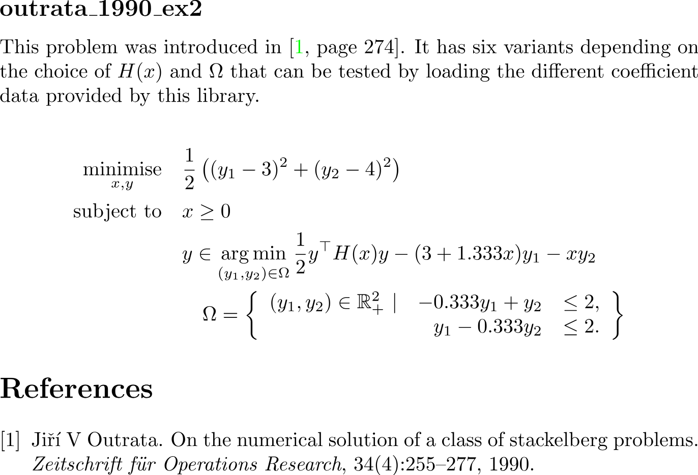
outrata_1990_ex2
Datasets
Description
On the Numerical Solution of a Class of Stackelberg Problems. Page 274. Example 1.Dimension
{
  "x": 1,
  "y": 2,
  "F": 1,
  "G": 1,
  "H": 0,
  "f": 1,
  "g": 4,
  "h": 0
}
Solution
{
  "optimality": "best_known",
  "x": [2.07],
  "y": [3,3],
  "F": 0.5,
  "f": -14.48793
}Description
On the Numerical Solution of a Class of Stackelberg Problems. Page 274. Example 2.Dimension
{
  "x": 1,
  "y": 2,
  "F": 1,
  "G": 1,
  "H": 0,
  "f": 1,
  "g": 4,
  "h": 0
}
Solution
{
  "optimality": "best_known",
  "x": [0],
  "y": [3,3],
  "F": 0.5,
  "f": -4.5
}Description
On the Numerical Solution of a Class of Stackelberg Problems. Page 274. Example 3.Dimension
{
  "x": 1,
  "y": 2,
  "F": 1,
  "G": 1,
  "H": 0,
  "f": 1,
  "g": 4,
  "h": 0
}
Solution
{
  "optimality": "best_known",
  "x": [3.456],
  "y": [1.707,2.569],
  "F": 1.859805,
  "f": -10.9309787632
}Description
On the Numerical Solution of a Class of Stackelberg Problems. Page 274. Example 4.Dimension
{
  "x": 1,
  "y": 2,
  "F": 1,
  "G": 1,
  "H": 0,
  "f": 1,
  "g": 4,
  "h": 0
}
Solution
{
  "optimality": "best_known",
  "x": [2.498],
  "y": [3.632,2.8],
  "F": 0.919712,
  "f": -19.468645
}Description
On the Numerical Solution of a Class of Stackelberg Problems. Page 274. Example 5.Dimension
{
  "x": 1,
  "y": 2,
  "F": 1,
  "G": 1,
  "H": 0,
  "f": 1,
  "g": 4,
  "h": 0
}
Solution
{
  "optimality": "best_known",
  "x": [3.999],
  "y": [1.665,3.887],
  "F": 0.897497,
  "f": -14.9311126675
}$title outrata_1990_ex2
$onText
J.V. Outrata
On the numerical solution of a class of Stackelberg problems
Zeitschrift für Operations Research
Volume 34, pages 255–277, (1990)
$offText
variables obj_val_upper, obj_val_lower, x, y1, y2;
equations obj_eq_upper, obj_eq_lower, g1_lower, g2_lower;
* Objective functions
obj_eq_upper.. obj_val_upper =e= 0.5*(sqr(y1 - 3) + sqr(y2 - 4));
obj_eq_lower.. obj_val_lower =e= 0.5*(y1+y2)*(y1+y2) - (3+ 0.333*x)*y1 - x*y2;
* Lower-level constraints
g1_lower.. -0.333*y1 + y2 =l= 2;
g2_lower.. y1 - 0.333*y_2 =l= 2;
* Bounds
x.lo = 0;
y1.lo = 0;
y2.lo = 0;
* Solve
model outrata_1990_ex2 / all /;
$echo bilevel x min obj_val_lower y obj_eq_lower g1_lower g2_lower> "%emp.info%"
solve outrata_1990_ex2 using emp min obj_val_upper;\subsection{outrata\_1990\_ex2}
\label{subsec:outrata_1990_ex2}
% Description
This problem was introduced in~\cite[page 274]{outrata1990}.
It has six variants depending on the choice of $H(x)$ and $\Omega$ that can be tested by loading the different coefficient data provided by this library.
% Equation
\begin{flalign*}
\minimise_{x, y} \quad
& \frac{1}{2}\left( (y_1-3)^2 + (y_2-4)^2 \right) \\
\subjectto \quad
& x\geq0\\
& y \in \argmin_{(y_1, y_2)\in\Omega}
\frac{1}{2} y^\top H(x) y - (3 + 1.333x)y_1 - x y_2\\
&\quad \Omega =
\left\{
\begin{array}{lrl}
(y_1, y_2)\in\R^2_{+}\ |
&-0.333y_1 + y_2 &\leq 2,\\
&y_1 - 0.333y_2 &\leq 2.
\end{array}
\right\}
\end{flalign*}classdef outrata_1990_ex2
%{
J.V. Outrata
On the numerical solution of a class of Stackelberg problems
Zeitschrift für Operations Research
Volume 34, pages 255–277, (1990)
%}
properties(Constant)
name = 'outrata_1990_ex2';
category = 'textbook';
subcategory = '';
datasets = {
'outrata_1990_ex2a.json';
'outrata_1990_ex2b.json';
'outrata_1990_ex2c.json';
'outrata_1990_ex2d.json';
'outrata_1990_ex2e.json';
'outrata_1990_ex2f.json';
};
paths = fullfile('bolib3', 'data', 'nonlinear', outrata_1990_ex2.datasets);
end
methods(Static)
% Upper-level objective function (quadratic)
% minimise 1/2 ((y1 - 3)^2 + (y2 - 4)^2)
function val = F(~, y, ~)
val = 0.5*((y(1) - 3)^2 + (y(2) - 4)^2);
end
% Upper-level inequality constraints (bounds)
% x >= 0
function val = G(x, ~, ~)
val = x(:);
end
% Upper-level equality constraints (none)
function val = H(~, ~, ~)
val = [];
end
% Lower-level objective function (nonconvex)
function val = f(x, y, data)
H_matrix = data.H_matrix + x*data.H_matrix_x_coefficients;
val = 0.5*(y'*H_matrix*y) - (3 + 1.333*x)*y(1) - x*y(2);
end
% Lower-level inequality constraints (quadratic)
% + (0.333 - 0.1x)y1 - y2 + x >= 0,
% - y1 + (0.333 + 0.1x)y2 + 2 >= 0,
% y1 >= 0,
% y2 >= 0.
function val = g(x, y, data)
y_coef = [
[0.333, -1];
[-1, 0.333]
];
val = [
y_coef*y + x*data.ineq_xy_coefficients*y + x*data.ineq_x_coefficients + data.ineq_constant;
y
];
end
% Lower-level equality constraints (none)
function val = h(~, ~, ~)
val = [];
end
% This bilevel program must be parameterized by data.
function data = read_data(filepath)
% Read JSON file
fid = fopen(filepath, 'r');
raw = fread(fid, inf, 'uint8=>char')';
fclose(fid);
data = jsondecode(raw);
% Define required keys and expected shapes
required_fields = {
'H_matrix', [2, 2];
'H_matrix_x_coefficients', [2, 2];
'ineq_xy_coefficients', [2, 2];
'ineq_x_coefficients', [2, 1];
'ineq_constant', [2, 1];
};
% Validate and convert each field
for i = 1:size(required_fields, 1)
key = required_fields{i, 1};
expected_shape = required_fields{i, 2};
if ~isfield(data, key)
error('Missing required field "%s" in "%s".', key, filepath);
end
% Validate numeric
if ~isnumeric(data.(key))
error('Field "%s" should be numeric.', key);
end
% Validate dimensions
if ~isequal(size(data.(key)), expected_shape)
error('Field "%s" should have dimensions [%d %d].', ...
key, expected_shape(1), expected_shape(2));
end
end
end
% Key are the function/variable names
% Values are their dimension
function n = dimension(key, ~)
n = dictionary( ...
'x', 1, ...
'y', 2, ...
'F', 1, ...
'G', 1, ...
'H', 0, ...
'f', 1, ...
'g', 4, ...
'h', 0 ...
);
if isKey(n,key)
n = n(key);
end
end
end
endimport json
import os.path
from bolib3 import np
"""
J.V. Outrata
On the numerical solution of a class of Stackelberg problems
Zeitschrift für Operations Research
Volume 34, pages 255–277, (1990)
"""
# Properties
name: str = "outrata_1990_ex2"
category: str = "textbook"
subcategory: str = ""
datasets: list = [
"outrata_1990_ex2a.json",
"outrata_1990_ex2b.json",
"outrata_1990_ex2c.json",
"outrata_1990_ex2d.json",
"outrata_1990_ex2e.json",
"outrata_1990_ex2f.json",
]
paths: list = [
os.path.join('bolib3', 'data', 'nonlinear', d) for d in datasets
]
# Methods
def F(x, y, data=None):
"""
Upper-level objective function (quadratic)
minimise 1/2 ((y1 - 3)^2 + (y2 - 4)^2)
"""
return 0.5*((y[0] - 3)**2 + (y[1] - 4)**2)
def G(x, y, data=None):
"""
Upper-level inequality constraints (bounds)
x >= 0
"""
return x
def H(x, y, data=None):
"""
Upper-level equality constraints (none)
"""
return np.empty(0)
def f(x, y, data: dict):
"""
Lower-level objective function (nonconvex)
"""
H_matrix = data['H_matrix'] + x[0]*data['H_matrix_x_coefficients']
return 0.5*np.dot(y, np.dot(H_matrix, y)) - (3 + 1.333*x[0])*y[0] - x[0]*y[1]
def g(x, y, data: dict):
"""
Lower-level inequality constraints (quadratic)
+ (0.333 - 0.1x)y1 - y2 + x >= 0,
- y1 + (0.333 + 0.1x)y2 + 2 >= 0,
y1 >= 0,
y2 >= 0.
"""
xy_coef = data["ineq_xy_coefficients"]
x_coef = data["ineq_x_coefficients"]
constant = data["ineq_constant"]
y_coef = np.array([
[0.333, -1],
[-1, 0.333]
])
return np.concatenate([
np.dot(y_coef, y) + x[0]*np.dot(xy_coef, y) + x[0]*x_coef + constant,
y
])
def h(x, y, data=None):
"""
Lower-level equality constraints (none)
"""
return np.empty(0)
def read_data(filepath):
"""
This bilevel program must be parameterized by data.
"""
with open(filepath, 'r') as f:
data = json.load(f)
# Validate as cast to numpy array
for key, shape in (
("H_matrix", (2, 2)),
("H_matrix_x_coefficients", (2, 2)),
("ineq_xy_coefficients", (2, 2)),
("ineq_x_coefficients", (2,)),
("ineq_constant", (2,)),
):
assert key in data, f"Missing required field \"{key}\" in '{filepath}'."
data[key] = np.array(data[key])
assert data[key].shape == shape, f"Field \"{key}\" should have dimensions {shape}."
return data
def dimension(key='', data=None):
"""
If the argument 'key' is not specified, then:
- a dictionary mapping variable/function names (str) to the corresponding dimension (int) is returned.
If the first argument 'key' is specified, then:
- a single integer representing the dimension of the variable/function with the name {key} is returned.
"""
n = {
"x": 1, # Upper-level variables
"y": 2, # Lower-level variables
"F": 1, # Upper-level objective functions
"G": 1, # Upper-level inequality constraints
"H": 0, # Upper-level equality constraints
"f": 1, # Lower-level objective functions
"g": 4, # Lower-level inequality constraints
"h": 0, # Lower-level equality constraints
}
if key in n:
return n[key]
return n