Added 18/06/2025
Transportation
dantzig_3_3
Dimension
{
  "x": 3,
  "y": 6,
  "F": 1,
  "G": 3,
  "H": 0,
  "f": 1,
  "g": 5,
  "h": 0
}
Solution
{
  "optimality": "stationary",
  "x": [325,304.9057,320.0943],
  "y": [45.0943,304.9057,0,279.9057,0,320.0943],
  "F": 21052.84678498,
  "G": [0,4.9057,45.0943],
  "H": [],
  "f": 1778.9717100000003,
  "g": [0,50,0,0,0],
  "h": []
}$title Transportation model with variable demand function using bilevel programming (TRANSBP,SEQ=26)
$onText
Dantzig's original transportation model TRNSPORT (in GAMS Model Library) is
reformulated using EMP's bilevel programming.
Dantzig, G B, Chapter 3.3. In Linear Programming and Extensions.
Princeton University Press, Princeton, New Jersey, 1963.
Additional features:
The fixed demand b(j) is replaced by a function:
g(j) = max(b(j),y(j))
with an outer objective function that tries to force y to be close to a
target value (400). The max function is modeled using Variational Inequalties.
The original trnsport model is the lower level problem.
Contributor: Michael Ferris, December 2009
$offText
Parameter report(*,*,*) summary report;
Sets
i canning plants / seattle, san-diego /
j markets / new-york, chicago, topeka / ;
Parameters
a(i) capacity of plant i in cases
/ seattle 350
san-diego 600 /
b(j) demand at market j in cases
/ new-york 325
chicago 300
topeka 275 / ;
Table d(i,j) distance in thousands of miles
new-york chicago topeka
seattle 2.5 1.7 1.8
san-diego 2.5 1.8 1.4 ;
Scalar f freight in dollars per case per thousand miles /90/ ;
Parameter c(i,j) transport cost in thousands of dollars per case ;
c(i,j) = f * d(i,j) / 1000 ;
Variables
x(i,j) shipment quantities in cases
z total transportation costs in thousands of dollars
g(j) generated demand;
Positive Variable x ;
Equations
cost define objective function
supply(i) observe supply limit at plant i
demand(j) satisfy demand at market j ;
cost .. z =e= sum((i,j), c(i,j)*x(i,j)) ;
supply(i) .. sum(j, x(i,j)) =l= a(i) ;
* --- Note: the fixed the demand b(j) was replaced by a variable demand g(j)
demand(j) .. sum(i, x(i,j)) =g= g(j) ;
Model transport /all/ ;
* --- Now we solve the original fixed price trnsport model
g.fx(j) = b(j);
Solve transport using lp minimizing z ;
report(i,j,'fixed') = x.l(i,j);
Variables
obj,
y(j) 'external demand function';
Equation
outerobj,
extdem(j);
outerobj.. obj =e= sum(j, sqr((y(j) - 400)/b(j)));
extdem(j).. g(j) =g= y(j);
model emp bilevel trnsport model / all /;
g.up(j) = inf; g.lo(j) = b(j);
* use the EMP info file to define the model
file fx / '%emp.info%' /;
put fx 'bilevel y' /;
put ' min z x cost supply demand' /;
putclose ' vi extdem g' /;
* --- Now we solve the bilevel trnsport model using EMP
solve emp us emp min obj;
report(i,j,"bilevel") = x.l(i,j);
Display report;\subsection{dantzig\_3\_3}
\label{subsec:dantzig_3_3}
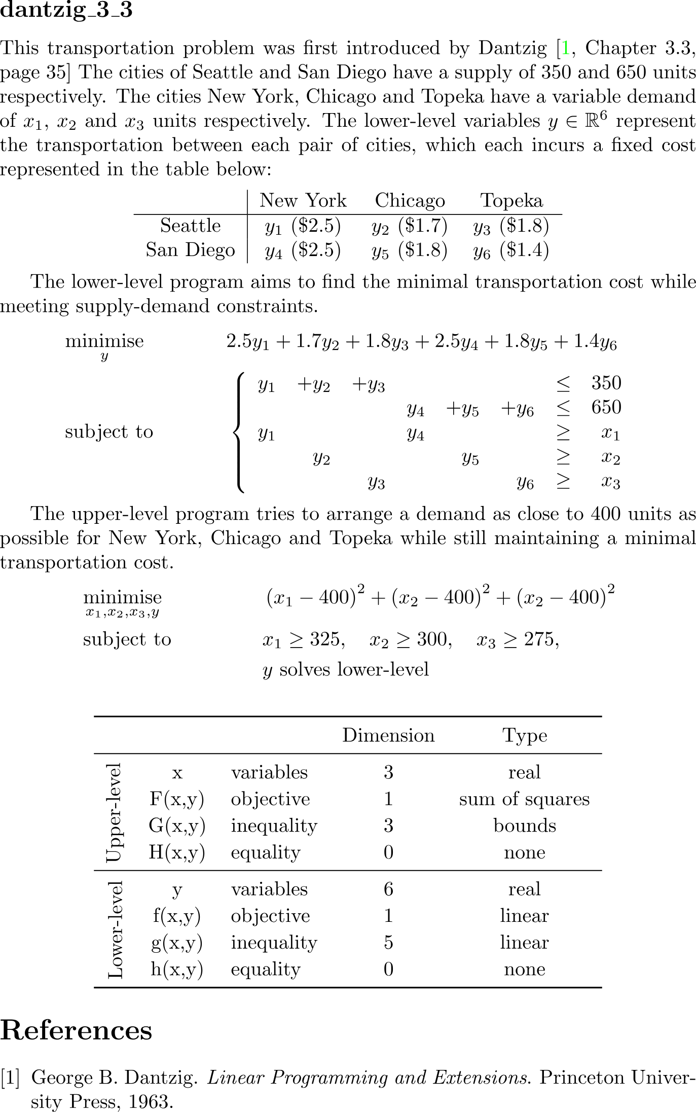
This transportation problem was first introduced by Dantzig~\cite[Chapter 3.3, page 35]{Dantzig1963}
The cities of Seattle and San Diego have a supply of 350 and 650 units respectively.
The cities New York, Chicago and Topeka have a variable demand of $x_1$, $x_2$ and $x_3$ units respectively.
The lower-level variables $y\in\R^6$ represent the transportation between each pair of cities, which each incurs a fixed cost represented in the table below:
\begin{center}
\begin{tabular}{c | c c c}
& New York & Chicago & Topeka\\
\hline
Seattle & $y_1\ (\$2.5)$ & $y_2\ (\$1.7)$ & $y_3\ (\$1.8)$ \\
San Diego & $y_4\ (\$2.5)$ & $y_5\ (\$1.8)$ & $y_6\ (\$1.4)$ \\
\end{tabular}
\end{center}
The lower-level program aims to find the minimal transportation cost while meeting supply-demand constraints.
\begin{align*}
&\minimise_{y}\quad&
&2.5 y_1 + 1.7 y_2 + 1.8 y_3 + 2.5 y_4 + 1.8 y_5 + 1.4 y_6\\
&\subjectto&
&\left\{
\begin{array}{rrrrrrrrcr}
y_1 & +y_2 & +y_3 & & & &\leq&350\\
& & & y_4 & +y_5 & +y_6 &\leq&650\\
y_1 & & & y_4 & & &\geq&x_1\\
& y_2 & & & y_5 & &\geq&x_2\\
& & y_3 & & & y_6 &\geq&x_3
\end{array}
\right.
\end{align*}
The upper-level program tries to arrange a demand as close to 400 units as possible for New York, Chicago and Topeka while still maintaining a minimal transportation cost.
\begin{align*}
&\minimise_{x_1, x_2, x_3, y}\quad&
&\left(x_1-400\right)^2 + \left(x_2-400\right)^2 + \left(x_2-400\right)^2\\
&\subjectto&
& x_1 \geq 325,\quad x_2 \geq 300,\quad x_3 \geq 275,\\
&&& y \text{ solves lower-level}
\end{align*}classdef dantzig_3_3
%{
Reference:
George B. Dantzig.
Linear Programming and Extensions.
Princeton University Press, 1963.
Chapter 3.3 Transportation Problem, page 35.
%}
properties(Constant)
name = 'dantzig_3_3';
category = 'transportation';
subcategory = '';
datasets = {};
paths = {};
x0 = [325.0000; 304.9057; 320.0943];
y0 = [45.0943; 304.9057; 0.0; 279.9057; 0.0; 320.0943];
end
methods(Static)
% Upper-level objective function
function val = F(x, ~, ~)
val = sum((x-400).^2);
end
% Upper-level inequality constraints
function val = G(x, ~, ~)
val = x(:) - [325; 300; 275];
end
% Upper-level equality constraints
function val = H(~, ~, ~)
val = [];
end
% Lower-level objective function
function val = f(~, y, ~)
val = dot(y, [2.5; 1.7; 1.8; 2.5; 1.8; 1.4]);
end
% Lower-level inequality constraints
function val = g(x, y, ~)
val = [
350 - y(1) - y(2) - y(3);
650 - y(4) - y(5) - y(6);
y(1) + y(4) - x(1);
y(2) + y(5) - x(2);
y(3) + y(6) - x(3);
];
end
% Lower-level equality constraints
function val = h(~, ~, ~)
val = [];
end
% If the bilevel program is parameterized by data, this function should
% provide code to read data file and return an appropriate structure.
function val = read_data(~)
val = [];
end
% Key are the function/variable names
% Values are their dimension
function n = dimension(key, ~)
n = dictionary( ...
'x', 3, ...
'y', 6, ...
'F', 1, ...
'G', 3, ...
'H', 0, ...
'f', 1, ...
'g', 5, ...
'h', 0 ...
);
if isKey(n,key)
n = n(key);
end
end
end
end# import numpy as np
import autograd.numpy as np
"""
Reference:
George B. Dantzig.
Linear Programming and Extensions.
Princeton University Press, 1963.
Chapter 3.3 Transportation Problem, page 35.
"""
# Properties
name: str = 'dantzig_3_3'
category: str = 'transportation'
subcategory: str = ''
datasets: list = []
paths: list = []
# Methods
def F(x, y, data=None):
"""
Upper-level objective function
(sum of squares)
"""
return np.sum((x - 400)**2)
def G(x, y, data=None):
"""
Upper-level inequality constraints
(bounds)
"""
return x - np.array([325, 300, 275])
def H(x, y, data=None):
"""
Upper-level equality constraints
(none)
"""
return np.empty(0)
def f(x, y, data=None):
"""
Lower-level objective function
(linear)
"""
return np.dot(y, np.array([2.5, 1.7, 1.8, 2.5, 1.8, 1.4]))
def g(x, y, data=None):
"""
Lower-level inequality constraints
(linear)
"""
return np.array([
350 - y[0] - y[1] - y[2],
650 - y[3] - y[4] - y[5],
y[0] + y[3] - x[0],
y[1] + y[4] - x[1],
y[2] + y[5] - x[2],
])
def h(x, y, data=None):
"""
Lower-level equality constraints
(none)
"""
return np.empty(0)
def read_data(filepath=''):
"""
If the bilevel program is parameterized by data, this function should
provide code to read data file and return an appropriate python structure.
"""
pass
def feasible_point(data=None):
"""
Returns a feasible point (x0, y0) satisfying:
G(x0, y0) >= 0,
H(x0, y0) == 0,
g(x0, y0) >= 0,
h(x0, y0) == 0.
"""
x0 = np.array([325.0000, 304.9057, 320.0943])
y0 = np.array([45.0943, 304.9057, 0.0, 279.9057, 0.0, 320.0943])
return x0, y0
def dimension(key='', data=None):
"""
If the argument 'key' is not specified, then:
- a dictionary mapping variable/function names (str) to the corresponding dimension (int) is returned.
If the first argument 'key' is specified, then:
- a single integer representing the dimension of the variable/function with the name {key} is returned.
"""
n = {
"x": 3, # Upper-level variables
"y": 6, # Lower-level variables
"F": 1, # Upper-level objective functions
"G": 3, # Upper-level inequality constraints
"H": 0, # Upper-level equality constraints
"f": 1, # Lower-level objective functions
"g": 5, # Lower-level inequality constraints
"h": 0 # Lower-level equality constraints
}
if key in n:
return n[key]
return n