Added 30/06/2025
Machine Learning / classification
svm_linear
Datasets
Description
Antennas radar signals used to classify structure in the ionosphere.Dimension
{
  "x": 42,
  "y": 114,
  "F": 1,
  "G": 83,
  "H": 0,
  "f": 1,
  "g": 158,
  "h": 0
}
Solution
{
  "optimality": "stationary",
  "F": 29.761108000000004,
  "f": 8.607208151197177,
  "training_accuracy": 0.962,
  "validation_accuracy": 0.7073
}Description
Length and width of sepals and petals labelled by species.Dimension
{
  "x": 35,
  "y": 71,
  "F": 1,
  "G": 69,
  "H": 0,
  "f": 1,
  "g": 132,
  "h": 0
}
Solution
{
  "optimality": "stationary",
  "F": 0.261069,
  "f": 1.131094,
  "training_accuracy": 1,
  "validation_accuracy": 1
}Description
Linearly Separable 2d dataset.Dimension
{
  "x": 12,
  "y": 22,
  "F": 1,
  "G": 23,
  "H": 0,
  "f": 1,
  "g": 38,
  "h": 0
}
Solution
{
  "optimality": "global",
  "F": 0,
  "f": 0.6064,
  "training_accuracy": 1,
  "validation_accuracy": 1
}Description
Coordinates sampled from two interweaving crescent moons.Dimension
{
  "x": 20,
  "y": 38,
  "F": 1,
  "G": 39,
  "H": 0,
  "f": 1,
  "g": 70,
  "h": 0
}
Solution
{
  "optimality": "stationary",
  "F": 6.60688,
  "f": 68.661357,
  "training_accuracy": 0.8,
  "validation_accuracy": 0.7895
}\subsection{svm\_linear}
\label{subsec:svm_linear}
% Data
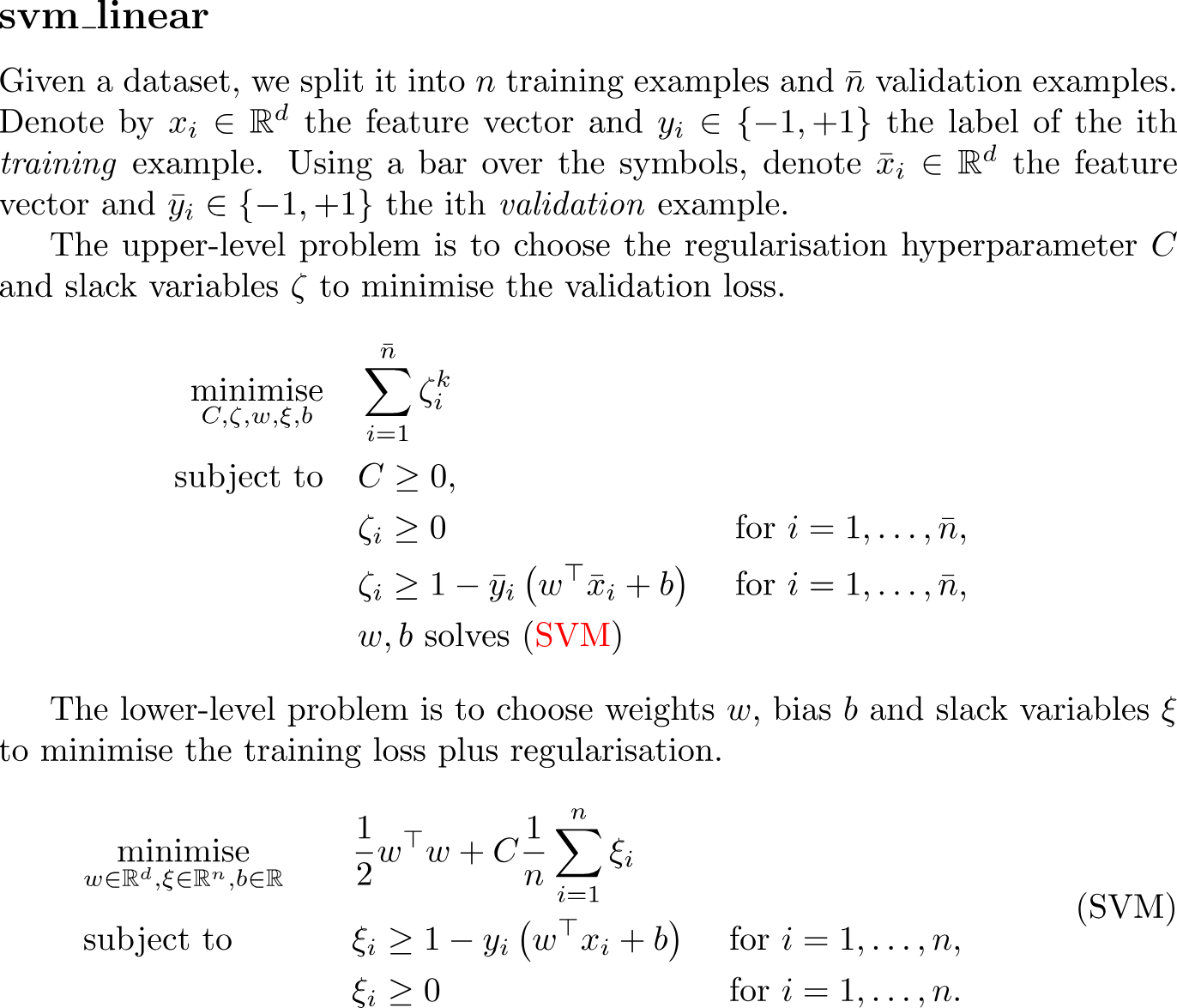
Given a dataset, we split it into $n$ training examples and $\bar{n}$ validation examples. Denote by $x_i\in\R^d$ the feature vector and $y_i\in\{-1,+1\}$ the label of the ith \emph{training} example. Using a bar over the symbols, denote $\bar{x}_i\in\R^d$ the feature vector and $\bar{y}_i\in\{-1,+1\}$ the ith \emph{validation} example.
% Upper-level problem
The upper-level problem is to choose the regularisation hyperparameter $C$ and slack variables $\zeta$ to minimise the validation loss.
\begin{equation*}
\begin{aligned}
\minimise_{C, \zeta, w, \xi, b} \quad
&\sum_{i=1}^{\bar{n}} \zeta_i^k&
\\
\subjectto \quad
&C \geq 0, & \\
&\zeta_i\geq 0& &\text{ for } i=1,\dots,\bar{n},& \\
&\zeta_i\geq 1 - \bar{y}_i \left(w^\top \bar{x}_{i}+b\right)& &\text{ for } i=1,\dots,\bar{n},& \\
&w,b \text{ solves \eqref{eq:svm_linear}}&
\end{aligned}
\end{equation*}
% Lower-level problem
The lower-level problem is to choose weights $w$, bias $b$ and slack variables $\xi$ to minimise the training loss plus regularisation.
\begin{align}
\label{eq:svm_linear}
\tag{SVM}
\begin{aligned}
&\minimise_{w\in\R^d,\xi\in\R^n,b\in\R}\quad &
&\frac{1}{2}w^{\top}w+C \frac{1}{n} \sum_{i=1}^{n}{\xi_{i}}&
\\
&\subjectto \quad &
&\xi_{i} \geq 1-y_{i}\left(w^\top x_{i}+b\right)&
&\text{ for } i=1,\dots,n,&
\\
&&
& \xi_i \geq0&
&\text{ for } i=1,\dots,n.&
\end{aligned}
\end{align}classdef svm_linear
%{
Linear Support Vector Machine (SVM)
===================================
The upper-level program seeks to choose x = [C, zeta] to minimise validation error.
The lower-level program seeks to choose y = [b, w, xi] to minimise training error.
Use the table below and svm_linear.pdf to reference variable names.
| Variable | Shape | Note |
| --------------- | ------------- | ------------------------------------------- |
| train_features | (n_train, d) | E.g. [[1.6,0.4], [4.7,1.5], [1.3,0.2], ...] |
| train_labels | (n_train,) | E.g. [+1, -1, +1, ...] |
| val_features | (n_val, d) | |
| val_features | (n_val,) | |
| | | |
| w | (d,) | Weights |
| b | (1,) | Bias |
| C | (1,) | Regularization hyperparameter |
| xi | (n_train,) | Slack variables for training hinge loss |
| zeta | (n_val,) | Slack variables for training hinge loss |
%}
properties(Constant)
name = 'svm_linear';
category = 'machine_learning';
subcategory = 'classification';
train_val_split = 0.66
datasets = {
'classification_ionosphere.csv';
'classification_iris.csv';
'classification_linearly_separable30.csv';
'classification_moons54.csv';
'classification_palmer.csv';
};
paths = fullfile('bolib3', 'data', 'classification', svm_linear.datasets);
end
methods(Static)
% //==================================================\\
% || F ||
% \\==================================================//
% Upper-level objective function (linear)
function val = F(x, ~, ~)
zeta = x(2:end);
val = sum(zeta);
end
% //==================================================\\
% || G ||
% \\==================================================//
% Upper-level inequality constraints (linear)
% C >= 0
% zeta_i >= 0
% zeta_i >= 1 - y_i (w^T x_i + b)
function val = G(x, y, data)
% Split variables
[C, zeta, b, w, ~] = svm_linear.variable_split(x, y, data);
% Compute validation hinge loss
% val_features has size (n_val x d)
% w has size (d x 1)
val_hinge_loss = 1 - data.val_labels .* (data.val_features * w + b);
% Combine constraints
val = [
C;
zeta;
zeta - val_hinge_loss
];
end
% //==================================================\\
% || H ||
% \\==================================================//
% Upper-level equality constraints
function val = H(~, ~, ~)
val = [];
end
% //==================================================\\
% || f ||
% \\==================================================//
% Lower-level objective function (quadratic)
% ||w||^2 + C * (1/n) * sum(xi)
function val = f(x, y, data)
% Reciprocal = 1 / n_train
reciprocal = data.reciprocal;
% Split variables
[C, ~, ~, w, xi] = svm_linear.variable_split(x, y, data);
% Compute objective
val = dot(w, w) + C * reciprocal * sum(xi);
end
% //==================================================\\
% || g ||
% \\==================================================//
% Lower-level inequality constraints (linear)
% xi >= 0
% xi >= 1 - y_i (w^T x_i + b)
function val = g(x, y, data)
% Training data
% Split variables
[~, ~, b, w, xi] = svm_linear.variable_split(x, y, data);
% Compute hinge loss for training data
train_hinge_loss = 1 - data.train_labels .* (data.train_features * w + b);
% Combine constraints
val = [
xi;
xi - train_hinge_loss
];
end
% //==================================================\\
% || h ||
% \\==================================================//
% Lower-level equality constraints
function val = h(~, ~, ~)
val = [];
end
% //==================================================\\
% || Variable Split ||
% \\==================================================//
% Splits the vectors x, y into their meaningful components.
% - Upper-level variables: X = [C; zeta_1; ...; zeta_n_val]
% - Lower-level variables: Y = [b; w_1; ...; w_d; xi_1; ...; xi_n_train]
function [C, zeta, b, w, xi] = variable_split(x, y, data)
% Upper-level variables
x = x(:);
C = x(1);
zeta = x(2:end);
% Lower-level variables
y = y(:);
b = y(1);
w = y(2:data.d+1);
xi = y(data.d+2:end);
end
% //==================================================\\
% || Evaluate ||
% \\==================================================//
% Calculates the training and validation accuracy scores.
function [train_accuracy, val_accuracy] = evaluate(x, y, data)
% Split decision variables
[C, ~, b, w, ~] = variable_split(x, y, data);
% Make predictions
train_predict = sign(data.train_features * w + b);
val_predict = sign(data.val_features * w + b);
% Compute accuracy
train_accuracy = sum(data.train_labels == train_predict) / data.n_train;
val_accuracy = sum(data.val_labels == val_predict) / data.n_val;
% Display if verbose
if verbose
fprintf('C (hyperparameter): %.2e\n', C);
fprintf('Training accuracy: %.2f%%\n', train_accuracy * 100);
fprintf('Validation accuracy: %.2f%%\n', val_accuracy * 100);
end
end
% //==================================================\\
% || Read Data ||
% \\==================================================//
% Reads data from a CSV file and splits it into training and validation.
% - The CSV file must have a header row.
% - The first column must contain +1/-1 labels.
% - The remaining columns are features.
% - Splits the data according to the 'train_val_split' property.
function data = read_data(filepath)
% Read CSV
options = detectImportOptions(filepath);
data_table = readtable(filepath, options);
% Extract labels and features
labels = data_table{:,1};
features = data_table{:,2:end};
% Dimensions
n_total = size(features, 1);
d = size(features, 2);
% Assertions
if ~all(ismember(labels, [-1, 1]))
error('Data contains labels other than -1 and +1');
end
if size(labels, 1) ~= n_total
error('Labels and features must have same number of rows');
end
% Split dataset
n_train = floor(n_total * svm_linear.train_val_split);
n_val = ceil(n_total * (1 - svm_linear.train_val_split));
train_features = features(1:n_train, :);
train_labels = labels(1:n_train);
val_features = features(n_train+1:end, :);
val_labels = labels(n_train+1:end);
% Store results in struct
data = struct();
data.file = filepath;
data.d = d;
data.n_val = n_val;
data.n_train = n_train;
data.reciprocal = 1 / n_train;
data.train_features = train_features;
data.train_labels = train_labels;
data.val_features = val_features;
data.val_labels = val_labels;
end
% //==================================================\\
% || Dimensions ||
% \\==================================================//
% Key are the function/variable names
% Values are their dimension
function n = dimension(key, data)
n = dictionary( ...
'x', 1 + data.n_val, ...
'y', 1 + data.d + data.n_train, ...
'F', 1, ...
'G', 1 + 2*data.n_val, ...
'H', 0, ...
'f', 1, ...
'g', 2*data.n_train, ...
'h', 0 ...
);
if isKey(n,key)
n = n(key);
end
end
end
endimport os
import math
from bolib3 import np
import matplotlib.pyplot as plt
import pandas as pd
"""
Linear Support Vector Machine (SVM)
===================================
The upper-level program seeks to choose x = [C, zeta] to minimise validation error.
The lower-level program seeks to choose y = [b, w, xi] to minimise training error.
Use the table below and svm_linear.pdf to reference variable names.
| Variable | Shape | Note |
| --------------- | ------------- | ------------------------------------------- |
| train_features | (n_train, d) | E.g. [[1.6,0.4], [4.7,1.5], [1.3,0.2], ...] |
| train_labels | (n_train,) | E.g. [+1, -1, +1, ...] |
| val_features | (n_val, d) | |
| val_features | (n_val,) | |
| | | |
| w | (d,) | Weights |
| b | (1,) | Bias |
| C | (1,) | Regularization hyperparameter |
| xi | (n_train,) | Slack variables for training hinge loss |
| zeta | (n_val,) | Slack variables for training hinge loss |
"""
# Properties
name: str = "svm_linear"
category: str = "machine_learning"
subcategory: str = "classification"
train_val_split: float = 0.66
datasets: list = [
'classification_ionosphere.csv',
'classification_iris.csv',
'classification_linearly_separable30.csv',
'classification_moons54.csv',
'classification_palmer.csv'
]
paths = [
os.path.join("bolib3", "data", "classification", d) for d in datasets
]
# //==================================================\\
# || F ||
# \\==================================================//
def F(x, y, data):
"""
Upper-level objective function
(linear)
minimise sum_{i=1,...,n_val} zeta_i
"""
zeta = x[1:]
return np.sum(zeta)
# //==================================================\\
# || G ||
# \\==================================================//
def G(x, y, data):
"""
Upper-level inequality constraints
(linear)
C ≥ 0
ζi ≥ 0
ζi ≥ 1 − yi(w^T xi + b)
"""
# Validation data
val_labels, val_features = data['val_labels'], data['val_features']
# Decision variables
C, zeta, b, w, _ = variable_split(x, y, data)
# Calculate the validation hinge loss
val_hinge_loss = 1 - val_labels*(np.dot(w, np.transpose(val_features)) + b)
return np.concatenate([
[C],
zeta,
zeta - val_hinge_loss,
])
# //==================================================\\
# || H ||
# \\==================================================//
def H(x, y, data=None):
"""
Upper-level equality constraints
(none)
"""
return np.empty(0)
# //==================================================\\
# || f ||
# \\==================================================//
def f(x, y, data):
"""
Lower-level objective function
(quadratic)
||w||^2 + C 1/n Σ ξi
"""
# The reciprocal is 1/n where n is the number of training examples
reciprocal = data['reciprocal']
# Decision variables
C, zeta, b, w, xi = variable_split(x, y, data)
return np.dot(w, w) + C*reciprocal*np.sum(xi)
# //==================================================\\
# || g ||
# \\==================================================//
def g(x, y, data):
"""
Lower-level inequality constraints
(linear)
ξi ≥ 0
ξi ≥ 1 − yi(w⊤xi + b)
"""
# Training data
train_labels, train_features = data['train_labels'], data['train_features']
# Decision variables
C, zeta, b, w, xi = variable_split(x, y, data)
# Calculate the training hinge loss function
train_hinge_loss = 1 - train_labels*(np.dot(w, np.transpose(train_features)) + b)
return np.concatenate([
xi,
xi - train_hinge_loss
])
# //==================================================\\
# || h ||
# \\==================================================//
def h(x, y, data=None):
"""
Lower-level equality constraints
(none)
"""
return np.empty(0)
# //==================================================\\
# || Variable Split ||
# \\==================================================//
def variable_split(x, y, data):
"""
Splits the vectors x, y into their more meaningful components.
Upper-level variables: x = (C, ζ_1, ..., ζ_n_val).
Lower-level variables: y = (b, w_1, ..., w_d, ξ_1, ..., ξ_n_train).
"""
# Dimensions of the data
d = data['d']
# Decision variables
C = x[0]
zeta = x[1:]
b = y[0]
w = y[1:d + 1]
xi = y[d + 1:]
return C, zeta, b, w, xi
# //==================================================\\
# || Read Data ||
# \\==================================================//
def read_data(filepath=paths[0], verbose=False):
"""
Reads data from a csv file.
- First row should contain header names (e.g. 'label', 'feature1', 'feature2', ...)
- First column should contain +1/-1 labels (e.g. [+1, -1, -1, +1, ...])
Splits the data into training and validation
"""
# Read the csv
df = pd.read_csv(filepath)
# Index the features and label from the pandas dataframe
labels = np.array(df.iloc[:, 0].values)
features = np.array(df.iloc[:, 1:].values)
# Dimensions of the data
n_total = features.shape[0] # rows
d = features.shape[1] # columns
# Assertions
assert np.all(np.isin(labels, [-1, 1])), "Data contains labels other than -1 and +1"
assert labels.shape[0] == features.shape[0], "Labels and features must have same number of rows"
# Split the dataset in training and validation
n_train, n_val = math.floor(n_total*train_val_split), math.ceil(n_total*(1 - train_val_split))
train_features, train_labels = features[:n_train], labels[:n_train]
val_features, val_labels = features[n_train:], labels[n_train:]
# Form into a dictionary
data = {
"path": filepath,
"d": d,
"n_val": n_val,
"n_train": n_train,
"reciprocal": 1/n_train,
"train_features": train_features,
"train_labels": train_labels,
"val_features": val_features,
"val_labels": val_labels,
}
# Print to console
if verbose:
for key, value in data.items():
print(f"{key:<15}: {value if (isinstance(value, int) or isinstance(value, float)) else value.shape}")
# Return the data
return data
# //==================================================\\
# || Evaluate ||
# \\==================================================//
def evaluate(x, y, data, verbose=True):
"""
Calculates the training and validation accuracy scores.
"""
# Decision variables
C, zeta, b, w, xi = variable_split(x, y, data)
# Make predictions
train_predict = np.sign(np.dot(data['train_features'], w) + b)
val_predict = np.sign(np.dot(data['val_features'], w) + b)
# Measure accuracy
train_accuracy = np.sum(data['train_labels'] == train_predict)/data['n_train']
val_accuracy = np.sum(data['val_labels'] == val_predict)/data['n_val']
# Print to console
if verbose:
print(f"C (hyperparameter): {C:.2e}")
print(f"Training accuracy: {train_accuracy:.2%}")
print(f"Validation accuracy: {val_accuracy:.2%}")
# Return tuple[float, float]
return train_accuracy, val_accuracy
# //==================================================\\
# || Plot SVM Boundary ||
# \\==================================================//
def plot_svm_boundary(x, y, data, d0=0, d1=1, title="Bilevel svm_linear problem decision boundary"):
"""
(x, y): upper and lower level decision variables for the bilevel svm_linear problem
data: see read_data()
d0: Column index of the first feature to be plotted (horizontal axis)
d1: Column index of the second feature to be plotted (vertical axis)
title: Title of the plot
"""
# Decision variables
C, zeta, b, w, xi = variable_split(x, y, data)
# Extract training and validation data
train_features, train_labels = data['train_features'], data['train_labels']
val_features, val_labels = data['val_features'], data['val_labels']
# Set up the figure
plt.figure(figsize=(8, 6))
# Scatter training data
mask = train_labels == 1
plt.scatter(train_features[mask, d0], train_features[mask, d1], color='green', marker='o', label=f'Training (+1)')
plt.scatter(train_features[~mask, d0], train_features[~mask, d1], color='red', marker='o', label=f'Training (-1)')
# Scatter validation data
mask = val_labels == 1
plt.scatter(val_features[mask, d0], val_features[mask, d1], color='green', marker='x', label=f'Validation (+1)')
plt.scatter(val_features[~mask, d0], val_features[~mask, d1], color='red', marker='x', label=f'Validation (-1)')
# Create decision boundary and margins
d0_space = np.linspace(plt.xlim()[0], plt.xlim()[1], 200)
# fix the unused dims to their mean
d345 = list(i for i in range(data['train_features'].shape[1]) if i not in [d0, d1])
mean = np.dot(w[d345], np.mean(data['train_features'], axis=0)[d345])
# Decision boundary
plt.plot(d0_space, -(w[d0]*d0_space + mean + b)/w[d1], 'k-', label='Decision boundary')
# Margins
plt.plot(d0_space, -(w[d0]*d0_space + mean + b + 1)/w[d1], 'k--', label='Margin')
plt.plot(d0_space, -(w[d0]*d0_space + mean + b - 1)/w[d1], 'k--')
plt.legend()
plt.title(title)
plt.xlabel(f"Feature {d0}")
plt.ylabel(f"Feature {d1}")
plt.tight_layout()
plt.show()
# //==================================================\\
# || Dimension ||
# \\==================================================//
def dimension(key='', data=None):
"""
If the argument 'key' is not specified, then:
- a dictionary mapping variable/function names (str) to the corresponding dimension (int) is returned.
If the first argument 'key' is specified, then:
- a single integer representing the dimension of the variable/function with the name {key} is returned.
"""
assert data is not None, "The svm_linear must be parameterized by data"
# Dimensions of the data
d, n_val, n_train = data['d'], data['n_val'], data['n_train']
# Dimensions of the decision variables
n = {
"x": 1 + n_val, # Upper-level variables x = [C, zeta_1, ..., zeta_n]
"y": 1 + d + n_train, # Lower-level variables y = [b, w_1, ..., w_d, xi_1, ..., xi_n]
"F": 1,
"G": 1 + 2*n_val,
"H": 0,
"f": 1,
"g": 2*n_train,
"h": 0,
}
if key in n:
return n[key]
return n
# Feasible point for ionosphere dataset
x0 = np.array([
40.27, 2.87776, 0.0, 0.0, 0.05403, 0.625691, 0.0, 0.286515, 0.0, 0.0, 0.617832, 0.0, 0.0, 0.0, 2.161009, 0.706492,
1.08977, 1.713132, 0.0, 0.629926, 0.547302, 1.714907, 0.0, 0.0, 0.0, 1.008483, 0.0, 1.771606, 3.186846, 0.74349,
0.06487, 0.499154, 0.15101, 1.83496, 1.879876, 1.644198, 0.0, 0.0, 0.961719, 0.299985, 0.628953, 2.061592
])
y0 = np.array([
-1.16497, 0.464239, 0.0, 0.397513, -0.068354, 0.747696, 0.459217, 0.461731, 0.294408, -0.01772, 0.354079, 0.183116,
0.089647, -0.11211, 0.36672, 0.192438, -0.381318, -0.015473, 0.302549, 0.031944, 0.164399, 0.18765, -0.548938,
0.268507, -0.141875, 0.223904, 0.096494, -0.449633, 0.283959, -0.026194, 0.082053, 0.095415, -0.070464, -0.043594,
-0.464038, 0.0, 0.0, 0.547609, 0.0, 0.0, 0.231288, 0.0, 0.031851, 0.0, 1.108514, 0.136396, 0.0, 0.0, 0.523643,
0.353763, 0.0, 0.0, 0.0, 0.0, 0.306526, 0.0, 0.207194, 0.0, 0.0, 0.0, 0.0, 0.594968, 0.0, 0.0, 0.0, 0.0, 0.0, 0.0,
0.0, 0.0, 0.0, 0.0, 0.0, 0.0, 0.0, 0.0, 0.0, 0.0, 0.0, 0.0, 0.0, 0.0, 0.0, 0.0, 0.0, 0.0, 0.0, 0.0, 0.0, 1.715708,
0.457647, 0.0, 0.0, 0.0, 0.0, 0.0, 0.0, 0.0, 0.0, 0.888483, 0.844932, 0.0, 0.0, 0.0, 0.056951, 0.346067, 0.0,
0.074463, 2.428207, 0.0, 0.0, 0.0, 0.0, 0.0
])